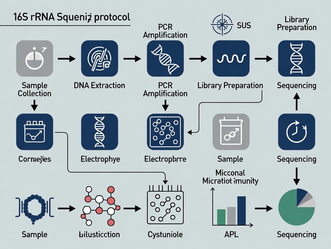
A Complete 16S rRNA Sequencing Protocol for Gut Microbiome Analysis: From Sample to Insights for Biomedical Research

Abstract

This comprehensive guide details a modern 16S rRNA gene sequencing protocol optimized for gut microbiome studies, tailored for researchers and drug development professionals. We cover the foundational principles of bacterial taxonomy, a step-by-step methodological workflow from sample collection through bioinformatics, common troubleshooting and optimization strategies for data quality, and a critical comparison with metagenomic sequencing. The article synthesizes best practices to generate robust, reproducible data for translational research, linking microbial community profiles to host physiology and therapeutic discovery.

Decoding the Gut Microbiome: Why 16S rRNA Sequencing is the Foundational Tool for Microbial Ecology

Application Notes & Protocols

1. Quantitative Overview of the Human Gut Microbiome

Table 1: Core Quantitative Characteristics of the Adult Human Gut Microbiota

Parameter	Typical Range / Value	Notes
Total Microbial Cells	~3.8 × 10^13	Roughly 1:1 ratio with human somatic cells.
Number of Bacterial Species	~300-500 prevalent species per individual	Thousands across the human population.
Dominant Phyla	Bacteroidetes (20-60%), Firmicutes (30-70%)	Relative abundance is highly variable and state-dependent.
Gene Count (Microbiome)	~3-5 million genes	Vastly exceeds the human genome (~20,000 genes).
Commonly Altered in Disease	Reduced diversity, altered Firmicutes/Bacteroidetes ratio, pathogen enrichment	Observed in IBD, Obesity, Type 2 Diabetes, etc.

Table 2: Association of Gut Microbiome Shifts with Specific Diseases

Disease/Condition	Reported Microbial Shift (Example Taxa)	Potential Functional Consequence
Inflammatory Bowel Disease (IBD)	↓ Faecalibacterium prausnitzii (anti-inflammatory), ↑ Escherichia coli	Reduced SCFA production, increased mucosal inflammation.
Obesity & Metabolic Syndrome	↓ Bacteroidetes, ↑ Firmicutes (in some studies); ↓ microbial gene richness	Increased energy harvest from diet; altered bile acid metabolism.
Type 2 Diabetes	↓ butyrate-producing bacteria (Roseburia, Eubacterium); ↑ Lactobacillus spp.	Impaired gut barrier function, systemic inflammation.
Colorectal Cancer (CRC)	↑ Fusobacterium nucleatum, ↑ Bacteroides fragilis (enterotoxigenic)	Promotion of cell proliferation, modulation of tumor immune microenvironment.

2. Core 16S rRNA Gene Sequencing Protocol for Gut Microbiome Profiling

Protocol: Fecal Sample Processing and 16S rRNA Gene Amplicon Sequencing (Illumina MiSeq Platform)

I. Sample Collection & Stabilization

• Collection: Collect fecal material using a sterile collection tube or commercial stool collection kit (e.g., with stabilizer buffer).
• Stabilization: Immediately suspend ~200 mg of fecal material in a DNA/RNA stabilizer (e.g., RNAlater, Zymo DNA/RNA Shield) to preserve microbial community structure. Store at -80°C.

II. DNA Extraction (Modified from the QIAamp PowerFecal Pro DNA Kit Protocol) Reagents/Equipment: Bead-beating tubes, vortex adapter, microcentrifuge, thermal shaker, magnetic rack.

• Homogenization: Thaw sample. Transfer 250 µL to a PowerBead Pro tube. Add 800 µL of CD1 solution.
• Bead Beating: Secure tubes on a vortex adapter. Vortex at maximum speed for 10 minutes.
• Incubation & Binding: Incubate at 65°C for 10 min with shaking (500 rpm). Centrifuge. Transfer supernatant to a clean tube.
• InhibitEx Technology: Add Inhibitor Removal Technology solution. Vortex, incubate at 4°C for 5 min, then centrifuge.
• DNA Binding: Transfer supernatant to a new tube with equal volume of CD2 binding solution. Load onto a MB Spin Column. Centrifuge.
• Wash: Wash with 700 µL of EA (ethanol-based) wash buffer, then 500 µL of C5 wash buffer. Dry column by centrifugation.
• Elution: Elute DNA in 50-100 µL of 10 mM Tris buffer, pH 8.5. Quantify using Qubit dsDNA HS Assay.

III. 16S rRNA Gene Amplification & Library Preparation Target Region: Hypervariable regions V3-V4 (~460 bp). Primers: 341F (5'-CCTACGGGNGGCWGCAG-3'), 806R (5'-GGACTACHVGGGTATCTAAT-3') with Illumina adapters.

• PCR Setup (25 µL):
  • 12.5 µL 2x KAPA HiFi HotStart ReadyMix
  • 5 µL Template DNA (5-20 ng)
  • 1.25 µL each Forward/Reverse Primer (1 µM final)
  • Nuclease-free water to 25 µL
• PCR Cycling:
  • 95°C for 3 min
  • 25 cycles: 95°C for 30s, 55°C for 30s, 72°C for 30s
  • 72°C for 5 min
  • Hold at 4°C.
• Clean-up: Purify amplicons using AMPure XP beads (0.8x ratio).
• Index PCR & Clean-up: Attach dual indices and Illumina sequencing adapters using Nextera XT Index Kit. Perform a second AMPure XP bead clean-up (0.8x ratio).
• Pooling & Quantification: Pool libraries equimolarly. Assess library size (Bioanalyzer) and quantify (qPCR). Load at 8-12 pM on an Illumina MiSeq with 2x300 bp v3 chemistry.

3. Data Analysis & Interpretation Workflow

Diagram Title: 16S rRNA Data Analysis Pipeline

4. Pathway: Microbial Short-Chain Fatty Acid (SCFA) Impact on Host

Diagram Title: SCFA Signaling Pathways in Host Health

5. The Scientist's Toolkit: Key Research Reagent Solutions

Table 3: Essential Materials for Gut Microbiome Research via 16S Sequencing

Item	Function/Application	Example Product/Kit
Stabilization Buffer	Preserves microbial community structure at point of collection, prevents DNA degradation.	Zymo DNA/RNA Shield, OMNIgene•GUT
Mechanical Lysis Beads	Ensures robust cell wall disruption of Gram-positive bacteria during DNA extraction.	Zirconia/Silica Beads (0.1 mm)
Inhibitor Removal Technology	Critical for removing PCR inhibitors (e.g., humic acids) common in fecal samples.	QIAamp PowerFecal Pro DNA Kit, DNeasy PowerSoil Pro Kit
High-Fidelity Polymerase	Reduces PCR amplification errors in target 16S region for accurate ASV calling.	KAPA HiFi HotStart, Q5 Hot Start
Size-Selective Beads	Purifies and size-selects amplicon libraries; removes primer dimers and contaminants.	AMPure XP Beads
Quantitative DNA Assay	Accurately quantifies low-concentration DNA without interference from RNA/contaminants.	Qubit dsDNA HS Assay
Curated 16S Reference Database	Provides high-quality aligned sequences for accurate taxonomic classification.	SILVA, Greengenes, RDP

Application Notes: Utility in Gut Microbiome Research

The 16S rRNA gene serves as the cornerstone for profiling the complex bacterial communities of the gut microbiome. Its application enables researchers to characterize microbial diversity, identify dysbiosis associated with disease states, and monitor the impact of therapeutic interventions, including drugs, probiotics, and diet.

Table 1: Key Regions of the 16S rRNA Gene Used for Gut Microbiome Sequencing

Hypervariable Region	Approximate Length (bp)	Resolution Level	Common Use Case in Gut Studies
V1-V2	~350	Genus to Species	Broad community profiling
V3-V4	~460	Genus (optimal)	Most common for gut microbiome (e.g., Illumina MiSeq)
V4	~250	Genus	High-throughput, cost-effective surveys
V4-V5	~400	Genus to Species	Balanced length and resolution
V6-V8	~400	Genus	Complementary to V3-V4

Table 2: Quantitative Output from a Typical 16S Gut Microbiome Study

Metric	Typical Range	Interpretation
Raw Sequences per Sample	50,000 - 100,000	Sequencing depth
Post-Quality Filtered Reads	70-90% of raw reads	Data quality
Observed ASVs/OTUs per Sample	100 - 500	Richness estimate
Alpha Diversity (Shannon Index)	3.0 - 6.0 (human gut)	Within-sample diversity
Beta Diversity (Weighted UniFrac)	PCoA plots; PERMANOVA p-value <0.05	Between-sample community differences

Detailed Experimental Protocols

Protocol 1: Library Preparation for 16S rRNA Gene Amplicons (V3-V4 Region)

Research Reagent Solutions Toolkit

Item	Function
DNA Extraction Kit (e.g., QIAamp PowerFecal Pro)	Lyses microbial cells and purifies genomic DNA from complex stool samples.
PCR Primers (e.g., 341F/805R)	Target conserved regions flanking the V3-V4 hypervariable zone for specific amplification.
High-Fidelity DNA Polymerase (e.g., KAPA HiFi)	Ensures accurate amplification with low error rates for faithful sequence representation.
Dual-Index Barcode Adapters (Illumina Nextera)	Attaches unique sample indices and Illumina sequencing adapters in a second PCR step.
Magnetic Bead Clean-up Kit (e.g., AMPure XP)	Purifies and size-selects amplicon libraries to remove primer dimers and contaminants.
Fluorometric Quantification Kit (e.g., Qubit dsDNA HS)	Precisely measures library concentration for accurate pooling.

Procedure:

• Genomic DNA Extraction: Extract total genomic DNA from 180-220 mg of homogenized stool using a dedicated kit. Include negative extraction controls.
• First-Stage PCR (Amplification):
  • Prepare 25 µL reactions: 12.5 µL 2X polymerase mix, 1 µL each of forward and reverse primers (10 µM), 1-10 ng template DNA.
  • Cycle conditions: 95°C for 3 min; 25 cycles of: 95°C for 30s, 55°C for 30s, 72°C for 30s; final extension 72°C for 5 min.
• Amplicon Purification: Clean PCR products using a magnetic bead protocol (0.8x bead-to-sample ratio). Elute in 30 µL nuclease-free water.
• Second-Stage PCR (Indexing): Attach unique dual indices and full adapters using a limited-cycle (8 cycles) PCR.
• Library Pooling & Clean-up: Quantify individual libraries, pool in equimolar ratios, and perform a final bead clean-up (0.9x ratio) before sequencing on an Illumina MiSeq (2x300 bp) or similar platform.

Protocol 2: Bioinformatic Analysis Pipeline (QIIME 2)

Procedure:

• Demultiplexing & Quality Control: Assign reads to samples based on barcodes. Import into QIIME 2 and denoise with DADA2 to correct errors and generate Amplicon Sequence Variants (ASVs).
• Taxonomic Assignment: Classify ASVs against a reference database (e.g., SILVA v138 or Greengenes2) using a trained classifier (e.g., naive Bayes).
• Diversity Analysis:
  • Alpha Diversity: Calculate metrics (Observed Features, Shannon, Faith PD) on rarefied feature tables.
  • Beta Diversity: Generate distance matrices (Unweighted/Weighted UniFrac, Bray-Curtis). Visualize via PCoA.
• Statistical Testing: Perform PERMANOVA on distance matrices to test for significant group differences. Use differential abundance tools (e.g, ANCOM-BC) to identify specific taxa associated with conditions.

Experimental Workflow & Conceptual Diagrams

Title: 16S rRNA Gut Microbiome Study Workflow

Title: 16S rRNA Data Bioinformatic Pipeline

Application Notes

In 16S rRNA gene sequencing for gut microbiome research, the selection of hypervariable region(s) (V1-V9) for PCR amplification is a critical primary step that directly influences taxonomic resolution, community composition profiles, and downstream biological interpretation. No single region universally captures the full diversity of the complex gut ecosystem; therefore, target selection is a balance of technical constraints and research goals.

Core Considerations for Region Selection:

• Resolution: Shorter regions (e.g., V4) offer higher sequencing depth and lower error rates but may lack species-level discrimination. Longer regions or multi-region approaches (e.g., V3-V4, V1-V3) provide finer taxonomic resolution but are more challenging for sequencing platforms.
• Database Coverage: The chosen region must align with well-annotated reference databases (e.g., SILVA, Greengenes, RDP). The V4 region is currently supported by the most comprehensive and curated reference sequences.
• Gut Microbiota Specificity: Certain regions are more effective for discriminating prevalent gut phyla. For example, the V3-V4 region is reliable for Firmicutes and Bacteroidetes, while V4-V5 can improve detection of Bifidobacterium and some Proteobacteria.
• Platform Compatibility: The total amplicon length must fit within the read length constraints of the sequencing platform (e.g., Illumina MiSeq, NovaSeq).

Table 1: Comparative Analysis of Key Hypervariable Regions for Gut Microbiome Studies

Target Region	Typical Amplicon Length	Primary Taxonomic Resolution	Strengths for Gut Microbiota	Key Limitations
V1-V3	~520 bp	Genus to Species	Good for Bifidobacterium, Lactobacillus; high discriminatory power.	Poor coverage for some Bacteroidetes; higher error rates in V1-V2.
V3-V4	~460 bp	Genus (some Species)	Robust for core phyla (Firmicutes/Bacteroidetes); widely used, standardized protocols.	May miss specific species-level markers present in other regions.
V4	~290 bp	Family to Genus	Excellent sequencing depth/depth, lowest error rate, best database support.	Limited species-level resolution for many taxa.
V4-V5	~400 bp	Genus	Improved for Bifidobacterium and Proteobacteria; good balance of length and resolution.	Less commonly used than V3-V4; slightly lower database curation.
Full-length (V1-V9)	~1500 bp	Species to Strain	Highest possible resolution; enables novel taxa discovery; gold standard.	Requires long-read sequencing (e.g., PacBio, Nanopore); higher cost/per-sample error.

Conclusion: For large-scale, cross-sectional studies focusing on community-level (beta-diversity) and family/genus-level shifts, the V3-V4 or V4 regions remain the benchmark due to robustness and reproducibility. For studies demanding higher resolution, such as strain tracking or precise pathogen identification, multi-region (V1-V3) or full-length 16S sequencing is recommended despite increased cost and complexity.

Protocol: 16S rRNA Gene Amplification & Library Preparation for the V3-V4 Region (Illumina MiSeq)

This protocol details the amplification of the 16S rRNA V3-V4 hypervariable region using dual-indexed primers, following the well-established Earth Microbiome Project guidelines.

I. Research Reagent Solutions & Essential Materials

Item	Function/Description
Primer Pair (341F/806R)	Forward (5'-CCTACGGGNGGCWGCAG-3') and Reverse (5'-GGACTACHVGGGTWTCTAAT-3') with overhang adapters for Nextera indexing.
High-Fidelity DNA Polymerase (e.g., KAPA HiFi)	Provides accurate amplification of complex microbial DNA templates with low error rates.
Nextera XT Index Kit (v2)	Contains unique dual-index (i7 & i5) primers for multiplexing hundreds of samples in a single run.
Magnetic Bead-based Cleanup System	For post-PCR purification and size selection to remove primer dimers and non-specific products.
Qubit dsDNA HS Assay Kit	Fluorometric quantification of DNA libraries to ensure accurate pooling.
Agilent Bioanalyzer/TapeStation	Fragment analyzer to verify amplicon library size distribution and quality.
Nuclease-free Water	Solvent for all dilution and reaction setup steps.

II. Step-by-Step Workflow Step 1: Genomic DNA Extraction & Quality Control

• Extract microbial genomic DNA from fecal samples using a bead-beating mechanical lysis kit to ensure robust cell wall disruption.
• Quantify DNA using Qubit. Verify integrity via 1% agarose gel or Fragment Analyzer.

Step 2: First-Stage PCR – Target Amplification

• Reaction Mix (25 µL):
  • Nuclease-free Water: 12.5 µL
  • 2X KAPA HiFi HotStart ReadyMix: 12.5 µL
  • Forward Primer (10 µM): 0.5 µL
  • Reverse Primer (10 µM): 0.5 µL
  • Template DNA (1-10 ng/µL): 2.0 µL
• Thermocycler Conditions:
  • 95°C for 3 min (initial denaturation)
  • 25 cycles of: 95°C for 30 sec, 55°C for 30 sec, 72°C for 30 sec
  • 72°C for 5 min (final extension)
  • Hold at 4°C.

Step 3: Purification of First-Stage PCR Products

• Clean amplicons using a magnetic bead clean-up protocol (0.8x bead-to-sample ratio).
• Elute in 25 µL of nuclease-free water or Tris buffer.

Step 4: Second-Stage PCR – Indexing & Library Construction

• Reaction Mix (25 µL):
  • Nuclease-free Water: 5 µL
  • 2X KAPA HiFi HotStart ReadyMix: 12.5 µL
  • Nextera XT Index Primer 1 (i7): 2.5 µL
  • Nextera XT Index Primer 2 (i5): 2.5 µL
  • Purified First-Stage PCR Product: 2.5 µL
• Thermocycler Conditions:
  • 95°C for 3 min
  • 8 cycles of: 95°C for 30 sec, 55°C for 30 sec, 72°C for 30 sec
  • 72°C for 5 min
  • Hold at 4°C.

Step 5: Final Library Purification, Quantification & Pooling

• Purify the indexed library with a magnetic bead clean-up (0.8x ratio).
• Quantify each library using Qubit.
• Check library fragment size (~630 bp) using Bioanalyzer.
• Normalize libraries to equimolar concentration (e.g., 4 nM).
• Pool normalized libraries together for a single sequencing run.

Step 6: Sequencing

• Denature and dilute the pooled library according to Illumina specifications.
• Load onto MiSeq Reagent Kit v3 (600-cycle) for 2x300 bp paired-end sequencing.

Diagram 1: 16S V3-V4 Amplicon Sequencing Workflow

Diagram 2: Hypervariable Region Selection Decision Logic

In 16S rRNA gene sequencing studies of the gut microbiome, clear research objectives are paramount. This document provides application notes and detailed protocols for analyzing alpha-diversity, beta-diversity, and taxonomic profiles. These objectives form the core analytical pillars for testing hypotheses related to disease association, drug response, and ecological dynamics within the gut microbial community.

Core Research Objectives & Quantitative Summaries

Table 1: Key Alpha-Diversity Indices

Index Name	Description	Formula/Model	Typical Value Range (Healthy Gut)	Interpretation in Gut Research
Observed ASVs/OTUs	Simple count of distinct taxonomic units.	S = count(ASV)	200 - 1000	Lower counts often associated with dysbiosis or disease states.
Shannon Index (H')	Measures richness and evenness.	H' = -Σ(pi * ln(pi))	3.0 - 7.0	Decrease indicates reduced diversity and potential instability.
Faith's Phylogenetic Diversity (PD)	Incorporates evolutionary distance.	Sum of branch lengths in phylogenetic tree.	15 - 50	Provides an evolutionary perspective on community richness.
Pielou's Evenness (J')	Assesses uniformity of species abundances.	J' = H' / ln(S)	0.7 - 0.9	Lower evenness suggests dominance by fewer taxa.

Table 2: Beta-Diversity Distance Metrics

Metric	Type (Qualitative/Quantitative)	Formula/Algorithm	Primary Use Case
Jaccard Distance	Qualitative (Presence/Absence)	1 - (	A∩B	/	A∪B	)	Detecting large-scale compositional shifts.
Bray-Curtis Dissimilarity	Quantitative (Abundance)	1 - (2*Σ min(Ni, Nj) / (ΣNi + ΣNj))	Most common for comparing community structure.
Weighted UniFrac	Quantitative & Phylogenetic	(Σ branches (b_i *	piA - piB	)) / (Σ branches (bi * (piA + p_iB)))	Detecting changes in abundant, phylogenetically related taxa.
Unweighted UniFrac	Qualitative & Phylogenetic	(Σ branches (bi * I(piA, piB))) / (Σ branches bi)	Sensitive to rare taxa and deep phylogenetic changes.

Table 3: Taxonomic Profiling & Abundance Ranges

Taxonomic Rank	Key Phyla in Gut (Typical Relative Abundance %)	Common Genera of Interest	Notes on Functional Relevance
Phylum	Bacteroidetes (20-60%), Firmicutes (30-70%), Actinobacteria (1-10%), Proteobacteria (<1-5%)	Bacteroides, Prevotella	Firmicutes/Bacteroidetes ratio often investigated.
Genus	Bacteroides (5-30%), Faecalibacterium (2-15%), Bifidobacterium (0.1-10%), Ruminococcus (1-5%)	Akkermansia, Roseburia	Faecalibacterium prausnitzii is a key butyrate producer.
Species	Often inferred via ASVs; exact abundances are protocol-dependent.	Species-level resolution is limited with V3-V4 16S regions.

Detailed Experimental Protocols

Protocol 1: Alpha-Diversity Analysis Workflow

Objective: To calculate and statistically compare within-sample diversity indices across experimental groups (e.g., Control vs. Treated).

• Input: Rarefied ASV/OTU table (e.g., 10,000 sequences per sample).
• Software: QIIME 2 (2024.5), R with phyloseq/vegan.
• Steps: a. Rarefaction: Subsample all samples to an even sequencing depth using qiime feature-table rarefy. b. Calculation: Compute indices (Observed, Shannon, Faith's PD) via qiime diversity alpha. c. Visualization: Generate rarefaction curves to confirm sufficient sequencing depth. d. Statistical Testing: Perform non-parametric Kruskal-Wallis test between groups. Apply false discovery rate (FDR) correction for multiple comparisons.
• Output: Box plots for each index; p-value table.

Protocol 2: Beta-Diversity Analysis Workflow

Objective: To assess between-sample compositional differences and test for group separation.

• Input: Rarefied ASV table and rooted phylogenetic tree.
• Distance Matrix Calculation: Generate Bray-Curtis and (Un)Weighted UniFrac matrices using qiime diversity beta.
• Ordination: Perform Principal Coordinates Analysis (PCoA) on the distance matrix.
• Statistical Testing: Conduct Permutational Multivariate Analysis of Variance (PERMANOVA) using qiime diversity adonis with 9999 permutations to test for significant group differences.
• Visualization: Plot PCoA results (e.g., PC1 vs. PC2) colored by experimental group.

Protocol 3: Taxonomic Composition Analysis

Objective: To determine relative abundances of taxa and perform differential abundance testing.

• Taxonomic Assignment: Use a pre-trained classifier (e.g., SILVA 138.1 or Greengenes2 2022.10) with qiime feature-classifier classify-sklearn.
• Bar Plot Creation: Collapse frequencies at the desired taxonomic level (e.g., Phylum) and visualize using qiime taxa barplot.
• Differential Abundance Analysis: a. Tool: Use ANCOM-BC2 (in R) or q2-gneiss for compositional-aware testing. b. Procedure: Apply model to compare groups, accounting for library size and compositionality bias. c. Output: List of differentially abundant taxa with log-fold changes and adjusted p-values (W-statistic for ANCOM-BC2).

Visual Workflows and Relationships

Title: 16S Data Analysis Objectives & Workflows

Title: Linking Hypothesis to Analysis Objectives

The Scientist's Toolkit: Research Reagent Solutions

Table 4: Essential Materials for 16S rRNA Sequencing & Analysis

Item	Function/Description	Example Product/Kit (Research Use Only)
Stool Collection & Stabilization Kit	Preserves microbial DNA at point of collection, inhibiting degradation.	OMNIgene•GUT, Zymo DNA/RNA Shield Fecal Collection Tube
Microbial DNA Isolation Kit	Efficiently lyses Gram+ bacteria and purifies PCR-inhibitor-free DNA.	QIAamp PowerFecal Pro DNA Kit, DNeasy PowerSoil Pro Kit
16S rRNA Gene PCR Primers	Amplifies hypervariable regions (e.g., V3-V4) for Illumina sequencing.	341F/806R, adapted for Illumina overhang addition.
High-Fidelity PCR Master Mix	Reduces amplification bias and errors during library construction.	KAPA HiFi HotStart ReadyMix, Q5 High-Fidelity DNA Polymerase
Index & Adapter Kit	Adds unique sample barcodes and Illumina flow cell adapters.	Illumina Nextera XT Index Kit v2, IDT for Illumina UD Indexes
Sequencing Standard	Validates run performance and aids in cross-study comparison.	ZymoBIOMICS Microbial Community Standard
Bioinformatics Pipeline	Processes raw sequences into ASVs/OTUs and taxonomic assignments.	QIIME 2, DADA2 (via R), MOTHUR
Reference Database	Provides curated taxonomy and aligned sequences for classification.	SILVA 138.1, Greengenes2 2022.10, RDP classifier
Positive Control DNA	Confirms PCR and sequencing steps function correctly.	ZymoBIOMICS Spike-in Control I (Low Microbial Load)
Emedastine Difumarate	Emedastine Difumarate, CAS:87233-62-3, MF:C25H34N4O9, MW:534.6 g/mol	Chemical Reagent
Irbesartan hydrochloride	Irbesartan Hydrochloride	Research-grade Irbesartan hydrochloride, an angiotensin II receptor blocker. For Research Use Only. Not for human or veterinary diagnostic or therapeutic use.

Before embarking on a 16S rRNA sequencing project to characterize the gut microbiome, rigorous preparatory steps are non-negotiable. The validity of findings linking microbiota to health, disease, or therapeutic response hinges on a robust study design, ethical compliance, and appropriate statistical power. This document outlines the essential pre-sequencing framework.

Ethical Considerations and Sample Acquisition

Ethical approval from an Institutional Review Board (IRB) or Ethics Committee is mandatory for human studies. Key protocols include:

Protocol 2.1: Informed Consent for Fecal Sample Collection

• Document Preparation: Develop a consent form detailing the study's purpose, procedures, risks, benefits, and data handling (including public repository deposition of anonymized sequences).
• Data Anonymization: Assign a unique study ID to each participant immediately upon collection. Separate the key linking IDs to personal information in a password-protected file.
• Sample Collection Kit: Provide participants with a sterile collection tube (e.g., DNA/RNA Shield Fecal Collection Tube) containing a stabilizer to preserve microbial composition at ambient temperature.
• Instructions: Provide clear written instructions for home collection, including avoiding collection during active gastrointestinal infection or within 4 weeks of antibiotic/probiotic use.
• Storage: Upon receipt, log samples and store at -80°C until DNA extraction.

Study Design Frameworks

The choice of design directly influences the experimental and analytical approach.

Table 1: Common Study Designs for 16S rRNA Gut Microbiome Research

Design Type	Key Characteristics	Best For	Statistical Consideration
Cross-Sectional	Single time point sampling of different groups.	Comparing healthy vs. diseased cohorts, or different dietary groups.	Controls must be matched for major confounders (age, BMI, sex).
Longitudinal	Repeated sampling from the same subjects over time.	Tracking microbiome changes in response to an intervention (drug, diet) or disease progression.	Requires repeated measures models. Account for dropout rates.
Paired Design	Samples are naturally paired (e.g., pre- and post-intervention in the same individual).	Measuring the direct effect of a treatment within subjects. Increases statistical power.	Use paired statistical tests (e.g., Wilcoxon signed-rank).

Title: Study Design Selection for Microbiome Research

Sample Size Calculation and Power Analysis

Underpowered studies are a major cause of irreproducible results. Calculations for microbiome studies often focus on alpha-diversity metrics or differential abundance.

Protocol 4.1: Sample Size Calculation Using Shannon Index A commonly used protocol based on comparing alpha diversity between two groups.

• Define Parameters:

  • Primary Metric: Shannon Diversity Index.
  • Effect Size (Δ): Minimum meaningful difference in mean Shannon Index. Pilot data or literature (e.g., Δ = 0.5) is required.
  • Standard Deviation (σ): Estimate of within-group standard deviation of the Shannon Index from pilot data or published studies.
  • Significance Level (α): Typically 0.05.
  • Power (1-β): Typically 0.80 or 0.90.

• Calculation Formula: For a two-sample t-test, the approximate sample size per group (n) is: n = 2 * ( (Z{1-α/2} + Z{1-β})^2 * σ^2 ) / Δ^2 Where Z is the critical value from the standard normal distribution.

• Adjustment: Increase calculated n by 15-20% to account for potential sample loss, failed sequencing, or contamination.

• Utilize Software: Perform calculation using G*Power, R (pwr package), or online calculators.

Table 2: Example Sample Size Calculations for a Two-Group Comparison (α=0.05, Power=0.80)

Effect Size (Δ)	Within-Group SD (σ)	Sample Size per Group (n)	Total Samples (2n)
0.5 (Moderate)	0.4	~21	42
0.8 (Large)	0.5	~16	32
0.3 (Small)	0.35	~27	54

Title: Sample Size Calculation Workflow

The Scientist's Toolkit: Research Reagent Solutions

Table 3: Essential Materials for Pre-Sequencing Phase

Item	Function & Rationale
Stabilized Fecal Collection Kit (e.g., Zymo DNA/RNA Shield, OMNIgene•GUT)	Preserves microbial genomic material at room temperature, preventing shifts in community structure post-collection and during transport.
Meta-analysis of Published 16S Data	Informs realistic effect size (Δ) and variance (σ) for power calculations when pilot data is unavailable.
Statistical Power Software (G*Power, R pwr, HMP)	Calculates necessary sample size to detect a specified effect with given confidence, preventing underpowered studies.
Sample Tracking LIMS (Laboratory Information Management System)	Manages de-identified participant metadata, sample IDs, and storage locations, ensuring chain of custody and preventing sample mix-ups.
Ethics Protocol Template	Provides a framework for drafting consent forms and IRB applications specific to human microbiome research, addressing data sharing and privacy.
Confounder Questionnaire	Standardized form to capture critical metadata (diet, medication, health status) essential for downstream statistical control and subgroup analysis.
Jaconine hydrochloride	Jaconine hydrochloride, CAS:7251-11-8, MF:C18H27Cl2NO6, MW:424.3 g/mol
3-Hydroxyhippuric acid	3-Hydroxyhippuric acid, CAS:3682-17-5, MF:C9H9NO3, MW:179.17 g/mol

Step-by-Step 16S rRNA Protocol: From Sample Collection to Sequence Data for Translational Research

Within the framework of a comprehensive thesis on 16S rRNA sequencing for gut microbiome research, the initial phase of sample collection and stabilization is paramount. The integrity of nucleic acids and microbial community structure from the moment of collection directly dictates the validity of downstream sequencing data. This document provides detailed application notes and protocols for fecal and intestinal mucosal samples, ensuring the preservation of microbial composition for accurate taxonomic profiling.

Critical Parameters for Sample Integrity

The choice of stabilization method significantly impacts the observed microbial community. The following table summarizes key quantitative findings from recent studies comparing common stabilization approaches for fecal samples.

Table 1: Impact of Stabilization Method on Fecal Microbial Community Integrity

Stabilization Method	Room Temp Stability (vs. Immediate -80°C)	Key Microbial Biases Reported	Optimal Storage Post-Stabilization	Reference (Example)
Immediate Freezing (-80°C)	Gold Standard; N/A	Minimal bias if frozen immediately.	Long-term at -80°C.	Gorvitovskaya et al., 2016
Commercially Available Stabilization Buffers (e.g., OMNIgene•GUT, RNAlater)	7-14 days stable.	May alter Firmicutes/Bacteroidetes ratio; reduces Gram-positive lysis.	Room temp (buffer-specific), then -80°C after mixing.	Vogtmann et al., 2017
95% Ethanol	24 hours stable.	Can cause selective loss of certain taxa; effective for DNA but not RNA.	-80°C after 24h at RT.	Hale et al., 2015
No Stabilizer (Air Drying/FTA cards)	Variable (days to weeks).	Significant biases; not recommended for community profiling.	Room temp, dry.	Sinha et al., 2016

Table 2: Mucosal Biopsy Collection & Stabilization Considerations

Parameter	Recommendation	Rationale
Biopsy Site	Specify precisely (e.g., terminal ileum, ascending/descending colon).	Microbial gradients exist along the GI tract.
Washing	Gently wash in sterile PBS or saline to remove luminal content.	Distinguishes mucosal-adherent vs. luminal communities.
Size	2-3 mm diameter (from standard forceps).	Adequate biomass while minimizing patient risk.
Immediate Processing	Snap-freeze in liquid Nâ‚‚ or place in >10x volume of stabilizer within 1 min.	Rapid changes occur ex vivo due to hypoxia and temperature shift.
Storage	Long-term at -80°C; avoid freeze-thaw cycles.	Preserves nucleic acid integrity.

Detailed Experimental Protocols

Protocol 1: Fecal Sample Collection & Stabilization Using Commercial Buffer

Objective: To collect and stabilize human fecal samples for 16S rRNA gene sequencing, preserving community structure at ambient temperature for transport.

Materials:

• Sterile collection container (without preservatives)
• Disposable spatula or spoon
• OMNIgene•GUT tube (DNA Genotek) or equivalent stabilizing buffer
• -80°C Freezer
• Laboratory vortex mixer
• Pre-labeled cryovials

Procedure:

• Collection: Collect fresh fecal sample into a sterile, dry container.
• Aliquoting: Using a sterile spatula, transfer approximately 100-200 mg of fecal material (pea-sized) into the tube containing stabilization buffer. Ensure the sample is submerged.
• Stabilization: Securely close the tube and shake vigorously for 10 seconds using a vortex mixer or by hand to homogenize the sample completely with the buffer.
• Transport/Short-term Storage: Stabilized samples can be stored at room temperature (up to 30°C) for 60 days as per manufacturer's guidelines for this buffer.
• Long-term Storage: For long-term preservation prior to DNA extraction, transfer 500 µL of the homogenized mixture to a cryovial and store at -80°C.

Protocol 2: Intestinal Mucosal Biopsy Collection & Snap-Freezing

Objective: To preserve the in vivo microbial and transcriptional profile of endoscopic mucosal biopsies.

Materials:

• Sterile endoscopic biopsy forceps
• Sterile phosphate-buffered saline (PBS)
• Petri dish
• Sterile surgical blades or scissors
• Cryovials, pre-labeled and chilled
• Liquid nitrogen or dry ice slurry
• Long-handled forceps

Procedure:

• Collection: Obtain biopsy using standard clinical endoscopic forceps.
• Washing: Immediately place biopsy in a Petri dish containing ice-cold, sterile PBS. Gently swirl to remove non-adherent luminal material.
• Trimming (Optional): If necessary, use a sterile blade to trim excess tissue, aiming for a consistent size (2-3 mm).
• Snap-Freezing: Briefly blot the biopsy on sterile filter paper to remove excess PBS. Quickly place the biopsy into a pre-chilled cryovial. Using long forceps, submerge the sealed cryovial in liquid nitrogen for a minimum of 30 seconds.
• Storage: Transfer and store vials at -80°C indefinitely. Do not allow samples to thaw.

Visualized Workflows

Fecal Sample Stabilization Decision Workflow

Mucosal Biopsy Snap-Freeze Protocol

The Scientist's Toolkit: Research Reagent Solutions

Table 3: Essential Materials for Optimal Sample Collection & Stabilization

Item	Function in Protocol	Key Consideration
OMNIgene•GUT (DNA Genotek)	Chemical stabilization of fecal microbial DNA at room temperature. Inhibits nuclease activity and growth.	Ideal for multi-center studies with non-refrigerated transport. May introduce buffer-specific bias.
RNAlater Stabilization Solution (Thermo Fisher)	Stabilizes and protects RNA (and DNA) in tissues/biopsies by penetrating cells and inactivating RNases.	For dual RNA/DNA analyses. Tissue must be <0.5 cm thick for adequate penetration.
Zymo Research DNA/RNA Shield	Inactivates nucleases and preserves microbial profile in fecal and tissue samples at room temperature.	Compatible with simultaneous DNA and RNA extraction.
Sterile PBS (pH 7.4)	Isotonic solution for washing mucosal biopsies to remove luminal contaminants.	Must be nuclease-free for RNA work; ice-cold to slow metabolic activity.
Pre-labeled Cryogenic Vials	Secure, leak-proof long-term storage of stabilized samples or snap-frozen tissues.	Use externally threaded vials; ensure labels are resistant to solvents, ice, and liquid Nâ‚‚.
Liquid Nitrogen or Dry Ice	Provides rapid cooling for "snap-freezing" of biopsies to instantly halt all biological activity.	Use appropriate PPE. For dry ice, use 95% ethanol or isopentane as slurry for faster freezing than dry ice alone.
Fluorescent brightener 24	Fluorescent brightener 24, CAS:12224-02-1, MF:C40H40N12Na4O16S4, MW:1165.0 g/mol	Chemical Reagent
Idalopirdine Hydrochloride	Idalopirdine Hydrochloride, CAS:467458-02-2, MF:C20H20ClF5N2O, MW:434.8 g/mol	Chemical Reagent

Within the broader thesis focusing on the development of a robust 16S rRNA gene sequencing protocol for gut microbiome research, Phase 2 addresses the most critical technical bottleneck: obtaining high-quality, inhibitor-free microbial DNA from complex gut matrices. The gut environment contains a plethora of PCR inhibitors, including bile salts, complex polysaccharides, hemoglobin derivatives, and dietary compounds, which can severely bias sequencing results by inhibiting downstream enzymatic steps. The optimization of DNA extraction and purification is therefore paramount for achieving accurate taxonomic profiling and reliable comparative analyses.

Current Challenges and Optimization Targets

Recent literature and empirical data highlight key variables influencing DNA yield, purity, and inhibitor content. The primary optimization targets are:

• Incomplete Cell Lysis: Gram-positive bacteria, spores, and archaea require more rigorous lysis conditions.
• Co-extraction of Inhibitors: Humic substances, bilirubin, and polysaccharides persist in extracts from fecal samples.
• DNA Shearing: Overly aggressive mechanical lysis can fragment DNA, affecting amplicon length.
• Bias Introduced by Kits: Different commercial kits exhibit taxonomic biases due to varied lysis efficiencies.

Quantitative Comparison of Commercial Kits and Methods

The following table summarizes performance metrics for four leading commercial kits and one enhanced in-house protocol, as reported in recent comparative studies (2023-2024).

Table 1: Performance Metrics of DNA Extraction Methods for Fecal Samples

Method / Commercial Kit	Avg. DNA Yield (ng/µg stool)	A260/A280 Purity	A260/A230 Purity	Reduction in Inhibitors (qPCR Efficiency)	Representative Cost per Sample	Key Bias Note
Kit A (Bead-beating + Silica Column)	45 ± 12	1.82 ± 0.05	2.05 ± 0.10	92%	$$$	Slight under-representation of Gram-positives
Kit B (Chemical Lysis + Magnetic Beads)	38 ± 10	1.90 ± 0.08	1.80 ± 0.15	85%	$$	Higher yield of Bacteroidetes
Kit C (Thermo-mechanical Lysis)	52 ± 15	1.78 ± 0.10	1.65 ± 0.20	78%	$$$$	Potential DNA shearing; high total yield
Kit D (Enzymatic + Column)	30 ± 8	1.95 ± 0.03	2.20 ± 0.08	95%	$$	Lower yield, highest purity
Optimized In-House Protocol	48 ± 14	1.85 ± 0.06	2.10 ± 0.10	96%	$	Customizable but labor-intensive

Detailed Optimized Protocol for Inhibitor-Rich Samples

Protocol 4.1: Enhanced Mechanical Lysis and Inhibitor Removal

Principle: This protocol combines rigorous mechanical disruption for broad taxonomic coverage with a post-extraction purification step specifically designed to remove common gut-derived PCR inhibitors.

Materials:

• Lysis Buffer: 500 mM NaCl, 50 mM Tris-HCl (pH 8.0), 50 mM EDTA, 4% SDS.
• Inhibitor Removal Solution: 3 M Guanidine Thiocyanate, 20 mM EDTA (pH 8.0), 0.1 M Potassium Acetate.
• Beads: A mixture of 0.1 mm zirconia/silica beads and 2 mm glass beads.
• Binding Matrix: Silica-coated magnetic beads.
• Wash Buffers: 80% Ethanol, 70% Ethanol.
• Elution Buffer: 10 mM Tris-HCl (pH 8.5) or nuclease-free water.

Procedure:

• Homogenization: Weigh 180-220 mg of frozen fecal sample into a 2 ml reinforced tube.
• Primary Lysis: Add 1 ml of pre-warmed (70°C) Lysis Buffer and the bead mixture. Secure tightly.
• Mechanical Disruption: Process in a high-speed bead beater for 3 cycles of 1 minute each, with 2-minute incubations on ice between cycles to prevent overheating.
• Inhibitor Binding: Centrifuge at 13,000 x g for 5 min. Transfer 800 µl of supernatant to a new tube. Add 200 µl of Inhibitor Removal Solution, vortex for 10 sec, and incubate on ice for 10 minutes. Centrifuge at 13,000 x g for 5 min.
• DNA Binding: Transfer 800 µl of the cleared supernatant to a tube containing 50 µl of resuspended silica magnetic beads. Incubate with rotation for 10 min at room temperature.
• Washing: Pellet beads on a magnet. Discard supernatant. Wash twice with 500 µl of 80% ethanol, followed by one wash with 500 µl of 70% ethanol. Air-dry for 5-10 min.
• Elution: Resuspend beads in 100 µl of pre-warmed Elution Buffer (55°C). Incubate for 5 min. Pellet beads and transfer the eluted DNA to a clean tube.
• Quality Control: Quantify using a fluorescence-based assay (e.g., Qubit). Assess purity via A260/A280 and A260/A230 ratios. Verify integrity and inhibitor removal via qPCR amplification of a 16S rRNA gene fragment using a standardized template.

Workflow and Pathway Visualizations

Diagram 1: Optimized DNA Extraction Workflow

Diagram 2: Gut Inhibitor Classes and Removal

The Scientist's Toolkit: Key Reagent Solutions

Table 2: Essential Research Reagents for DNA Extraction Optimization

Reagent / Material	Function in Protocol	Key Consideration
Zirconia/Silica Beads (0.1 mm)	Mechanical disruption of robust cell walls (Gram-positives, spores).	Superior durability and lysis efficiency compared to glass alone.
Guanidine Thiocyanate (GuSCN)	Chaotropic agent for inhibitor precipitation and nucleic acid binding.	Critical for removing humic acids and polyphenols. Handle with care.
Silica-Coated Magnetic Beads	Solid-phase reversible immobilization (SPRI) for DNA binding and washing.	Enables automation, reduces organic waste vs. spin columns.
PCR Inhibitor Removal Solution	Proprietary blends (e.g., with polyvinylpyrrolidone) to sequester inhibitors.	Used as a post-elution "clean-up" step for difficult samples.
Lysozyme & Proteinase K	Enzymatic lysis complementing mechanical methods.	Target peptidoglycan and proteins; require specific incubation temps.
PCR Efficiency Assay Kit	Quantitative measure of inhibitor carryover using a standardized DNA template.	Essential QC step before costly sequencing runs.
Syringaresinol diglucoside	Syringaresinol diglucoside, CAS:573-44-4, MF:C34H46O18, MW:742.7 g/mol	Chemical Reagent
Methylprednisolone Aceponate	Methylprednisolone Aceponate, CAS:86401-95-8, MF:C27H36O7, MW:472.6 g/mol	Chemical Reagent

Within the context of a comprehensive 16S rRNA gene sequencing protocol for gut microbiome research, the PCR amplification step is a critical source of bias that can distort the apparent microbial community structure. Biases introduced during primer design and amplification can lead to inaccurate taxonomic profiling, compromising downstream analyses and conclusions regarding dysbiosis or therapeutic response. This application note details strategies and protocols to minimize amplification bias, ensuring more representative and reproducible results for researchers, scientists, and drug development professionals.

PCR bias stems from both primer-template mismatches and amplification kinetics. The table below summarizes primary sources and their impacts.

Table 1: Primary Sources of PCR Bias in 16S rRNA Gene Amplification

Source of Bias	Mechanism	Impact on Community Profile
Primer-Template Mismatch	Variation in primer binding efficiency due to sequence polymorphisms in target sites.	Under-representation of taxa with mismatches; false negatives.
Number of PCR Cycles	Increased cycles exaggerate initial amplification efficiency differences.	Over-representation of initially favored templates; reduced correlation with true abundance.
Polymerase Choice	Different enzymes have varying processivity, fidelity, and mismatch tolerance.	Altered amplicon length distribution and community evenness.
Primer Dimer Formation	Non-specific primer-primer annealing consumes reagents.	Reduced target yield; introduction of non-target sequences.
Chimeric Sequence Formation	Incomplete extension products act as primers in subsequent cycles.	Generation of artifactual sequences mis-assigned to novel taxa.

Primer Design Guidelines for Hypervariable Regions

The selection of hypervariable region(s) (e.g., V3-V4, V4) and corresponding primers is foundational. Optimal primers should:

• Target conserved regions flanking the variable region.
• Exhibit broad coverage across the domain Bacteria (and/or Archaea if relevant).
• Minimize degeneracy while accounting for necessary variation to maintain coverage.
• Be evaluated in silico for coverage and mismatch analysis using current databases like SILVA or Greengenes.

Table 2: Commonly Used Primer Pairs for Gut Microbiome Studies (Updated)

Target Region	Primer Pair (Forward / Reverse)	Approx. Amplicon Length	Key Considerations for Bias Reduction
V4	515F (GTGYCAGCMGCCGCGGTAA) / 806R (GGACTACNVGGGTWTCTAAT)	~290 bp	High coverage of Bacteria & Archaea; widely adopted for Illumina platforms.
V3-V4	341F (CCTACGGGNGGCWGCAG) / 805R (GACTACHVGGGTATCTAATCC)	~465 bp	Provides greater taxonomic resolution; requires longer read sequencing.
V4-V5	515F (GTGYCAGCMGCCGCGGTAA) / 926R (CCGYCAATTYMTTTRAGTTT)	~410 bp	Alternative for higher resolution; requires optimization for some Firmicutes.

Detailed Protocol: Low-Bias PCR Amplification for 16S Libraries

Materials & Reagents

See "The Scientist's Toolkit" below for detailed list.

Procedure

• Template Preparation: Use standardized genomic DNA input (e.g., 1-10 ng) quantified by fluorometry. Include a negative control (nuclease-free water).
• Reaction Setup (25 µL):
  • 12.5 µL: High-fidelity, low-bias PCR Master Mix (e.g., KAPA HiFi, Q5)
  • 1.25 µL each: Forward and Reverse Primer (10 µM stock)
  • 1-5 µL: Template DNA (adjust volume so mass is consistent)
  • Nuclease-free water to 25 µL
• Thermocycling Conditions:
  • Initial Denaturation: 95°C for 3 min.
  • Amplification Cycles (25-30 cycles):
    • Denature: 95°C for 30 sec.
    • Anneal: 55°C (or Tm-optimized) for 30 sec.
    • Extend: 72°C for 30 sec/kb.
  • Final Extension: 72°C for 5 min.
  • Hold: 4°C.
  • Note: Do not exceed 30 cycles. Perform reactions in triplicate to mitigate stochastic early-cycle bias.
• Post-PCR Processing: Pool triplicate reactions. Purify amplicons using a size-selective magnetic bead clean-up (e.g., AMPure XP beads) to remove primer dimers and non-target fragments.
• Quality Control: Verify amplicon size and purity via microfluidic electrophoresis (e.g., Agilent Bioanalyzer, Fragment Analyzer).

Visualization of Workflow & Bias Mitigation Strategies

Bias Sources & Mitigation in 16S PCR Workflow

How PCR Cycles Exacerbate Primer Bias

The Scientist's Toolkit: Research Reagent Solutions

Table 3: Essential Materials for Low-Bias 16S rRNA PCR Amplification

Item	Example Product(s)	Function & Importance for Bias Reduction
High-Fidelity DNA Polymerase	KAPA HiFi HotStart, Q5 High-Fidelity, Platinum SuperFi II	High processivity and fidelity reduce misincorporation and chimeric sequence formation.
Low-Bias PCR Master Mix	AccuPrime Pfx, LongAmp Taq	Specifically optimized buffers/enzymes for balanced amplification of complex mixtures.
Validated Primer Panels	Earth Microbiome Project primers, Klindworth et al. 2013 primers	Pre-evaluated for broad phylogenetic coverage and minimal bias.
Magnetic Bead Clean-up	AMPure XP, SPRIselect	Size-selective purification removes primer dimers and non-target fragments.
Microfluidic QC System	Agilent Bioanalyzer, Fragment Analyzer	Accurate sizing and quantification of amplicon libraries prevent loading bias.
Fluorometric DNA Quant Kit	Qubit dsDNA HS Assay, PicoGreen	Accurate quantitation of initial gDNA and final library for input normalization.
m-PEG5-2-methylacrylate	m-PEG5-2-methylacrylate, MF:C15H28O7, MW:320.38 g/mol	Chemical Reagent
m-PEG6-2-methylacrylate	m-PEG6-2-methylacrylate, MF:C17H32O8, MW:364.4 g/mol	Chemical Reagent

Meticulous primer design and optimized, minimal-cycle PCR are non-negotiable steps for obtaining representative 16S rRNA gene amplicon data from complex gut microbiome samples. By adhering to the protocols and strategies outlined here—utilizing validated, broad-coverage primers, high-fidelity polymerases, and stringent cycle limits—researchers can significantly reduce technical bias, thereby increasing the biological accuracy and reproducibility of their sequencing data for robust research and drug development applications.

In the context of 16S rRNA sequencing for gut microbiome research, Phase 4 represents the critical transition from purified PCR amplicons to sequence-ready libraries. This phase determines data quality, multiplexing capacity, and compatibility with modern high-throughput sequencing platforms. The choice between short-read (Illumina) and long-read (PacBio) platforms involves trade-offs between read length, accuracy, cost, and throughput, directly impacting downstream taxonomic resolution and analysis.

Library Preparation & Indexing: Core Principles

Library preparation for 16S rRNA sequencing involves attaching platform-specific adapters and sample-specific indices (barcodes) to the amplicon target regions (e.g., V3-V4). Indexing allows for multiplexing—pooling dozens to hundreds of samples in a single sequencing run—dramatically reducing per-sample cost.

Key Considerations for 16S rRNA Studies

• Adapter Design: Must be compatible with the chosen sequencing platform.
• Dual Indexing: Using unique indices on both ends of the amplicon minimizes index hopping artifacts and increases multiplexing capacity.
• PCR Cycles: Optimized to minimize chimera formation and bias.
• Clean-up: Critical for removing primer-dimers, unused reagents, and short fragments.

Quantitative Comparison of Common Library Prep Kits

Table 1: Comparison of Representative 16S rRNA Library Prep Kits (2023-2024)

Kit Name (Manufacturer)	Target Region	Indexing Strategy	Avg. Hands-on Time	Recommended Input	Key Feature
Nextera XT Index Kit (Illumina)	Variable (user-defined)	Dual, 384 unique combinations	~2.5 hours	1 ng amplicon	Integrated tagmentation, fast protocol
16S Metagenomic Sequencing Library Prep (Illumina)	V3-V4	Dual, 96 index primers	~3.5 hours	10 ng genomic DNA	Includes target amplification & cleanup
SMRTbell Prep Kit 3.0 (PacBio)	Full-length 16S (V1-V9)	Dual, via barcoded primers	~4 hours	100-200 ng amplicon	Optimized for long-read circular consensus sequencing

Detailed Protocol: Dual-Indexed 16S V3-V4 Library Prep for Illumina

This protocol is adapted from the Illumina "16S Metagenomic Sequencing Library Preparation Guide" (Part #15044223 Rev. B).

A. Materials & Equipment:

• Purified 16S V3-V4 amplicons.
• KAPA HiFi HotStart ReadyMix (2X): High-fidelity polymerase for minimal bias.
• Illumina Nextera XT Index Kit (v2): Provides 384 unique dual index combinations.
• AMPure XP Beads: Magnetic beads for size selection and clean-up.
• Library Quantification Kit (e.g., Qubit dsDNA HS Assay): For accurate DNA concentration measurement.
• Bioanalyzer or TapeStation (Agilent): For library fragment size distribution analysis.
• Thermal cycler, magnetic stand, and microcentrifuge.

B. Procedure:

Step 1: Amplification with Indexing Primers

• Prepare the indexing PCR reaction on ice:
  • 2.5 µL of purified 16S amplicon.
  • 2.5 µL of Nextera XT Index Primer 1 (i7).
  • 2.5 µL of Nextera XT Index Primer 2 (i5).
  • 12.5 µL KAPA HiFi HotStart ReadyMix (2X).
  • Total Volume: 25 µL.
• Run the PCR:
  • 95°C for 3 min.
  • 8 cycles of: 95°C for 30 sec, 55°C for 30 sec, 72°C for 30 sec.
  • 72°C for 5 min.
  • Hold at 4°C.

Step 2: Clean-up with AMPure XP Beads (0.8X Ratio)

• Vortex AMPure XP beads to resuspend. Add 20 µL of beads (0.8X sample volume) to each 25 µL reaction. Mix thoroughly.
• Incubate at room temperature for 5 minutes.
• Place on a magnetic stand for 2 minutes until supernatant clears.
• Carefully remove and discard the supernatant.
• With tube on magnet, wash beads twice with 200 µL freshly prepared 80% ethanol.
• Air dry beads for 5 minutes. Remove from magnet.
• Resuspend dried beads in 27.5 µL of Resuspension Buffer (RSB). Incubate for 2 minutes.
• Place on magnet. Transfer 25 µL of cleared supernatant (containing indexed library) to a new tube.

Step 3: Library Validation & Quantification

• Quantify final library using Qubit dsDNA HS Assay.
• Assess library size distribution (~550-600 bp for V3-V4) using Agilent Bioanalyzer High Sensitivity DNA chip.
• Calculate library concentration in nM:
  • (Qubit concentration in ng/µL) / (library size in bp * 660) * 10^6 = nM.

Step 4: Pooling and Denaturation

• Dilute each indexed library to 4 nM in RSB.
• Combine equal volumes of each 4 nM library to create a pooled library.
• Denature the pooled library with NaOH per Illumina's standard denaturation protocol for loading onto the MiSeq or iSeq.

Modern Sequencing Platforms: Illumina vs. PacBio for 16S

Table 2: Platform Comparison for 16S rRNA Sequencing in Gut Microbiome Research

Parameter	Illumina MiSeq/iSeq	PacBio Sequel IIe/Revio
Read Technology	Short-read, sequencing-by-synthesis (SBS)	Long-read, Single Molecule Real-Time (SMRT) sequencing
Typical 16S Output	2x300 bp (paired-end)	Full-length gene (~1,500 bp) via Circular Consensus Sequencing (CCS)
Key Advantage	High throughput, low per-base cost, excellent accuracy (>99.9%)	Species- and strain-level resolution, eliminates PCR primer bias
Key Limitation	Short reads limit taxonomic resolution to genus level; chimera risk from PCR	Higher per-sample cost, lower throughput, requires more input DNA
Best Suited For	Large-scale cohort studies, genus-level community profiling	Studies requiring high taxonomic resolution, novel species discovery

The Scientist's Toolkit: Research Reagent Solutions

Table 3: Essential Reagents and Materials for Phase 4

Item	Function in Protocol	Example Product/Supplier
High-Fidelity PCR Mix	Attaches indices via limited-cycle PCR with minimal error	KAPA HiFi HotStart ReadyMix (Roche), Q5 Hot Start (NEB)
Dual Indexed Adapter Kit	Provides unique barcode combinations for sample multiplexing	Nextera XT Index Kit v2 (Illumina), IDT for Illumina UD Indexes
SPR/Bead-Based Cleanup Reagent	Size-selects and purifies libraries from primers and small fragments	AMPure XP Beads (Beckman Coulter), SPRIselect (Beckman)
Library Quantification Assay	Precisely measures double-stranded DNA concentration	Qubit dsDNA HS Assay Kit (Thermo Fisher)
Library Size QC Kit	Analyzes fragment size distribution to confirm correct library construction	Agilent High Sensitivity DNA Kit (Bioanalyzer/TapeStation)
Sequencing Control	Monitors run performance and aids in phasing/prephasing calculations	PhiX Control v3 (Illumina)
Ornithine-methotrexate	Ornithine-methotrexate, CAS:80407-73-4, MF:C20H25N9O3, MW:439.5 g/mol	Chemical Reagent
2-Aminobenzenesulfonic acid	2-Aminobenzenesulfonic acid, CAS:88-21-1, MF:C6H7NO3S, MW:173.19 g/mol	Chemical Reagent

Workflow and Conceptual Diagrams

Workflow: Library Prep Paths for Major Platforms

Platforms: Core Sequencing Technology Comparison

Within the comprehensive thesis on 16S rRNA gene sequencing protocols for gut microbiome research, the bioinformatics phase is critical for transforming raw sequencing data into biologically interpretable results. This section details the application of three predominant analytical workflows: DADA2/DeBlur for Amplicon Sequence Variant (ASV) inference, QIIME 2, and Mothur. The shift from Operational Taxonomic Units (OTUs) to ASVs offers higher resolution by distinguishing single-nucleotide differences, promising greater reproducibility in longitudinal studies of gut microbiota dynamics relevant to drug development.

The choice of pipeline influences downstream statistical results and ecological interpretations. The following table summarizes the core characteristics, inputs, and primary outputs of each featured workflow.

Table 1: Comparison of 16S rRNA Bioinformatics Pipelines

Feature	DADA2/DeBlur (ASV-based)	QIIME 2 (Framework)	Mothur (OTU-based)
Core Philosophy	Error-correction to infer exact biological sequences.	Modular, extensible platform for microbiome analysis.	Standardized, all-in-one pipeline for community ecology.
Output Unit	Amplicon Sequence Variants (ASVs).	Supports both ASVs (via plugins) and OTUs.	Predominantly Operational Taxonomic Units (OTUs).
Primary Method	Divisive partitioning, statistical error models (DADA2); positional error profiling (DeBlur).	Wraps multiple tools (e.g., DADA2, DeBlur, VSEARCH).	Distance-based clustering (e.g., average neighbor).
Key Strength	High-resolution, reproducible sequences without clustering.	Reproducibility via artifacts & metadata tracking, vast plugin ecosystem.	Highly standardized, follows the original Schloss SOP, excellent support for full-length 16S.
Typical Input	Demultiplexed, quality-filtered FASTQ files.	Raw FASTQ or imported data artifacts (.qza).	Multiplexed or demultiplexed FASTQ, and mapping file.
Computational Demand	Moderate to High.	Varies with plugins; generally moderate.	Low to Moderate.
Best Suited For	Studies requiring fine-scale differentiation (e.g., strain tracking).	Collaborative projects needing reproducibility and flexibility.	Studies comparing to legacy data or requiring strict SOP adherence.

Detailed Experimental Protocols

Protocol 1: DADA2 Workflow for ASV Inference

This protocol processes paired-end Illumina reads to generate a feature table of ASVs and their taxonomy.

Materials & Reagents:

• Software: R (v4.3.0+), DADA2 package (v1.30.0+).
• Input Data: Demultiplexed, primer-trimmed forward and reverse FASTQ files.
• Reference Databases: SILVA (v138) or Greengenes (v13_8) formatted for DADA2 (e.g., for taxonomy assignment).

Methodology:

• Filter and Trim: Quality filter reads based on expected errors (maxEE) and truncate at positions where median quality drops (e.g., truncLen=c(240,200)).

• Learn Error Rates: Model the error profile from the data.

• Dereplicate: Collapse identical reads.

• Sample Inference: Apply the core DADA algorithm to infer true sequences.

• Merge Paired Reads: Merge forward and reverse reads, removing mismatches.

• Construct Sequence Table: Build an ASV table (rows=samples, columns=ASVs).

• Remove Chimeras: Identify and remove bimera sequences.

• Taxonomy Assignment: Assign taxonomy using a naive Bayesian classifier against a reference database.

Protocol 2: QIIME 2 Core Analysis via DADA2 Plugin

QIIME 2 encapsulates analyses in reproducible, documented workflows.

Materials & Reagents:

• Software: QIIME 2 (v2024.5+), installed via Conda.
• Input Data: Manifest-formatted raw FASTQ files and sample metadata (TSV).
• Reference Data: QIIME 2-compatible taxonomy classifier (e.g., gg-13-8-99-515-806-nb-classifier.qza).

Methodology:

• Import Data: Create a QIIME 2 artifact.

• Denoise with DADA2: Generate ASV table, representative sequences, and denoising stats.

• Taxonomy Classification: Assign taxonomy using a pre-trained classifier.

• Generate Visualizations: Create interactive summaries.

Protocol 3: Mothur Standard Operating Procedure (SOP)

This protocol follows the Mothur MiSeq SOP for generating OTUs.

Materials & Reagents:

• Software: Mothur (v1.48.0+).
• Input Data: Multiplexed FASTQ files and a sample metadata file.
• Reference Files: Mothur-compatible reference alignment (e.g., SILVA reference alignment) and taxonomy file.

Methodology:

• Make Contigs: Combine paired-end reads into contigs.

• Screen Sequences: Align to reference and remove those not aligning in the correct region.

• Pre-cluster: Denoise sequences by merging near-identical reads.

• Chimera Removal: Identify chimeras using UCHIME.

• Classify Sequences: Assign taxonomy using the naive Bayesian classifier.

• Cluster into OTUs: Generate distance matrix and cluster sequences (e.g., at 97% similarity).

• Generate OTU Table: Classify OTUs and create a final shared file.

Visualizations

Title: 16S Pipeline Decision Flow

Title: DADA2 vs Mothur Workflow Comparison

The Scientist's Toolkit: Research Reagent Solutions

Table 2: Essential Bioinformatics Tools & Resources for 16S Analysis

Item	Function/Description	Example/Source
Reference Database	Provides curated phylogenetic and taxonomic framework for sequence classification.	SILVA, Greengenes, RDP.
Pre-trained Classifier	Machine-learning model for fast, accurate taxonomic assignment within a pipeline.	QIIME2 gg-13-8-99-nb-classifier.
Conda Environment	Manages isolated, reproducible software installations with specific version dependencies.	Miniconda/Anaconda distribution.
QIIME 2 Artifact (.qza)	Containerized data + provenance, ensuring full reproducibility of analysis steps.	Output from any QIIME 2 tool.
Denoising Algorithm	Statistically distinguishes biological sequences from sequencing errors to generate ASVs.	DADA2 (divisive), DeBlur (substitution).
Chimera Checking Tool	Identifies and removes artificial sequences formed from multiple parent sequences.	VSEARCH uchime_denovo, DADA2 removeBimeraDenovo.
Multiple Sequence Alignment (MSA) Tool	Aligns sequences for phylogenetic tree construction (more common in OTU pipelines).	MAFFT (in QIIME2), align.seqs in Mothur.
Metadata File (TSV)	Tab-separated file containing sample-associated variables (e.g., pH, treatment, host BMI) for downstream analysis.	Must follow QIIME 2 formatting guidelines.
Oxyphenisatin Acetate	Oxyphenisatin Acetate|CAS 115-33-3|Research Chemical	Oxyphenisatin acetate is a research chemical for cancer mechanism studies. This product is For Research Use Only and is not intended for diagnostic or personal use.
Paliperidone Palmitate	Paliperidone Palmitate	High-purity Paliperidone Palmitate, a long-acting antipsychotic reagent for schizophrenia research. For Research Use Only. Not for human use.

Downstream analysis of 16S rRNA sequencing data transforms processed amplicon sequence variant (ASV) or operational taxonomic unit (OTU) tables into biological insights. This phase involves statistical hypothesis testing, advanced visualization, and ecological interpretation within the context of gut microbiome research for therapeutic discovery.

Core Statistical Testing Frameworks

Statistical evaluation determines significant differences in microbial composition and function between experimental groups (e.g., treated vs. control, disease vs. healthy).

Table 1: Common Statistical Tests for 16S Microbiome Data

Analysis Goal	Statistical Test/Method	Key Assumptions	When to Use	Software/Package
Differential Abundance	DESeq2 (with count data)	Negative binomial distribution, sufficient replicates	Identifying specific taxa with significant abundance changes between groups	R: DESeq2, phyloseq
Beta Diversity Significance	Permutational Multivariate Analysis of Variance (PERMANOVA)	Similar multivariate spread among groups (homogeneity of dispersion)	Testing if overall microbial community structure differs between groups	R: vegan (adonis2)
Alpha Diversity Comparisons	Wilcoxon Rank-Sum / Kruskal-Wallis	Non-normal distribution of diversity indices	Comparing within-sample diversity (e.g., Shannon, Faith's PD) between groups	R: stats, ggplot2
Compositional Data Analysis	Analysis of Compositions of Microbiomes (ANCOM-BC)	Sparse log-contrast model, addresses compositionality	Robust differential abundance testing for compositional data	R: ANCOMBC
Correlation & Association	SparCC or FastSpar	Compositional, sparse correlations	Inferring robust microbial association networks	Python: SpiecEasi, R: SpiecEasi

Detailed Protocols for Key Analyses

Protocol 3.1: PERMANOVA for Beta Diversity

Objective: To statistically assess whether microbial community structures differ significantly between predefined groups.

Materials:

• Normalized or rarefied ASV/OTU table (samples x features)
• Sample metadata with grouping variable
• Pre-calculated distance matrix (e.g., Bray-Curtis, Unifrac)

Procedure:

• Load Data: Import distance matrix and metadata into R using phyloseq or vegan.
• Check Dispersion: Test homogeneity of group dispersions using betadisper() (vegan). A non-significant result is ideal.
• Run PERMANOVA: Execute adonis2(distance_matrix ~ Group_Variable, data = metadata, permutations = 9999).
• Interpret: A significant p-value (e.g., < 0.05) indicates overall community difference. Always report R² (variance explained).
• Post-hoc: If >2 groups, perform pairwise PERMANOVA with p-value adjustment (e.g., Bonferroni).

Protocol 3.2: Differential Abundance with DESeq2

Objective: Identify taxa whose abundances are significantly different between conditions.

Procedure:

• Prepare Data: Create a phyloseq object. Do NOT rarefy. Use raw count data.
• Run DESeq2:

• Shrinkage: Apply lfcShrink() for accurate log2 fold change estimates.
• Visualize: Generate MA-plots and volcano plots. Transform counts using varianceStabilizingTransformation for plotting.

Visualization Strategies

Table 2: Essential Visualizations for Data Interpretation

Visualization	Purpose	Key Aesthetics	Tool
Principal Coordinates Analysis (PCoA)	Visualize beta-diversity and sample clustering	Points colored by group, ellipses for confidence intervals	R: ggplot2 (with vegan/phyloseq)
Stacked Bar Plot (Taxonomic Composition)	Display relative abundance of major taxa across samples	Fill color by Genus/Phylum, x-axis as samples grouped by condition	R: phyloseq::plot_bar()
Heatmap (Clustered)	Visualize abundance patterns of significant taxa across samples	Z-score normalized abundance, row/column clustering	R: pheatmap, ComplexHeatmap
Linear Discriminant Analysis Effect Size (LEfSe) Plot	Highlight taxa most likely to explain differences between classes	Cladogram and bar plot of LDA scores	Python: Huttenhower Lab Galaxy, R: microbiomeMarker
Volcano Plot (Differential Abundance)	Contrast statistical significance vs. magnitude of change (log2 fold change)	-log10(padj) vs. log2FoldChange, colored by significance	R: EnhancedVolcano

Diagram: Downstream Analysis Workflow

Title: 16S Downstream Analysis Workflow

Diagram: Statistical Decision Pathway

Title: Statistical Test Selection Pathway

The Scientist's Toolkit: Research Reagent Solutions

Table 3: Essential Tools for Downstream Analysis

Item / Software	Category	Primary Function in Analysis
R (v4.3+) with RStudio	Programming Environment	Core platform for statistical computing and graphics.
phyloseq (v1.46)	R Package	Data structure and methods for organizing ASV table, taxonomy, metadata, and phylogenetic tree.
vegan (v2.6-6)	R Package	Community ecology package for PERMANOVA, diversity indices, and ordination (PCoA, NMDS).
DESeq2 (v1.42)	R Package	Differential abundance testing based on negative binomial generalized linear models.
QIIME 2 (v2024.5)	Pipeline/Platform	End-to-end analysis platform; used for generating core metrics and initial visualizations.
MicrobiomeAnalyst 2.0	Web Platform	User-friendly web-based tool for comprehensive statistical and visual analysis.
ggplot2 (v3.5)	R Package	Declarative grammar of graphics for creating publication-quality visualizations.
PICRUSt2 / BugBase	Bioinformatics Tool	Inferring metagenome functional content from 16S data and predicting phenotypic traits.
Git / GitHub	Version Control	Tracking code changes, collaboration, and ensuring reproducibility of the analysis.
FastSpar / SpiecEasi	Correlation Tool	Inferring robust, sparse microbial co-occurrence networks from compositional data.
Paramethasone Acetate	Paramethasone Acetate, CAS:1597-82-6, MF:C24H31FO6, MW:434.5 g/mol	Chemical Reagent
2-(1-hydroxypentyl)benzoic Acid	2-(1-hydroxypentyl)benzoic Acid, CAS:380905-48-6, MF:C12H16O3, MW:208.25 g/mol	Chemical Reagent

Data Interpretation in Gut Microbiome Research

Interpretation must move beyond statistical significance to biological relevance. Key considerations include:

• Effect Size: Report and interpret R² values (PERMANOVA) and log2 fold changes (Differential Abundance).
• Confounders: Adjust for covariates (e.g., age, BMI, diet) in statistical models where possible.
• Taxonomic Resolution: Interpret findings at the appropriate level (e.g., species-level inferences require high-resolution sequencing).
• Causality vs. Association: 16S data typically reveals associations; integrate with mechanistic studies (e.g., gnotobiotic models) for causal insight.
• Functional Context: Use predictive tools (PICRUSt2, Tax4Fun2) cautiously and validate key predictions with metabolomics or transcriptomics.
• Clinical Relevance: For drug development, link microbial signatures to host pathophysiology, biomarkers, or therapeutic response.

Troubleshooting Your 16S rRNA Data: Solving Common Pitfalls and Optimizing for Reproducibility

Addressing Low DNA Yield and Quality from Complex Gut Samples

Within the broader thesis on optimizing 16S rRNA sequencing protocols for gut microbiome research, a fundamental challenge is the reliable extraction of high-yield, high-quality microbial DNA from complex gut samples. These samples, including feces and intestinal biopsies, contain inhibitors like bile salts, polysaccharides, and host DNA, which compromise downstream sequencing accuracy and diversity representation. This application note details current methodologies and protocols to overcome these barriers.

The primary obstacles in DNA extraction from gut samples and their impacts are summarized below.

Table 1: Common Challenges in Gut Microbiome DNA Extraction

Challenge	Typical Impact on Yield	Typical Impact on Quality (A260/A280)	Downstream Effect on 16S Sequencing
High Inhibitor Content (e.g., bile salts)	Reduction of 40-70%	Skewed ratios (<1.6 or >2.0)	PCR inhibition, low library prep efficiency
Dominant Host DNA (biopsies)	Microbial DNA <10% of total	N/A (host DNA co-extracted)	Reduced microbial read depth, wasted sequencing
Variable Bacterial Lysis Efficiency	Yield variability up to 300% between species	Potential shearing from harsh methods	Bias in community representation
DNA Shearing	N/A	Fragment size <10 kbp	Poor performance in long-read sequencing

Table 2: Comparison of DNA Extraction Method Classes

Method Class	Avg. Yield (Feces)	Avg. A260/A280	Time (Hands-on)	Cost/Sample	Inhibitor Removal Efficacy
Phenol-Chloroform	High	1.7-1.9	High (>2 hrs)	Low	Moderate
Silica-column Kit	Moderate	1.8-2.0	Low (~30 min)	Moderate	High (with modifications)
Magnetic Bead Kit	Moderate-High	1.8-2.0	Low (~30 min)	Moderate-High	High
PTFE-based Kit	High	1.8-2.0	Moderate (~1 hr)	High	Very High

Detailed Experimental Protocols

Protocol 1: Enhanced Mechanical Lysis and Inhibitor Removal for Fecal Samples

This protocol modifies a commercial silica-column kit for maximal yield and purity.

Materials: See "The Scientist's Toolkit" below. Procedure:

• Homogenization: Weigh 180-220 mg of wet fecal material into a 2 ml screw-cap tube containing 1.4 mm ceramic beads and 1 ml of InhibitEX buffer/lysis solution. Homogenize in a bead-beater at 6.0 m/s for 45 seconds. Incubate at 95°C for 5 minutes.
• Inhibitor Binding: Centrifuge at 13,000 x g for 1 minute. Transfer up to 800 µl of supernatant to a new tube containing a proprietary inhibitor removal tablet (e.g., InhibitEX tablet). Vortex for 1 minute until fully suspended. Incubate at room temperature for 1 minute.
• Precipitation & Binding: Centrifuge at 13,000 x g for 3 minutes. Pipette up to 700 µl of supernatant into a new tube. Add 1 volume of binding buffer (e.g., AL buffer) and 1 volume of 100% ethanol. Mix by vortexing for 15 seconds.
• Column Purification: Transfer 700 µl of mixture to a silica-column. Centrifuge at 10,000 x g for 1 min. Discard flow-through. Repeat until all lysate is processed.
• Washes: Add 500 µl wash buffer 1 (AW1). Centrifuge at 10,000 x g for 1 min. Discard flow-through. Add 500 µl wash buffer 2 (AW2). Centrifuge at full speed for 3 min. Dry column by a final 1 min centrifugation.
• Elution: Place column in a clean 1.5 ml tube. Apply 50-100 µl of pre-heated (70°C) Tris-EDTA (TE) buffer or nuclease-free water to the membrane center. Incubate for 5 min at room temperature. Centrifuge at full speed for 1 min to elute DNA. Store at -20°C.

Protocol 2: Host DNA Depletion for Intestinal Biopsy Samples

This protocol uses a mild enzymatic pretreatment to reduce host cell lysis prior to microbial DNA extraction.

Materials: Collagenase, DNase I, Proteinase K, Phosphate-Buffered Saline (PBS), Microbial DNA extraction kit. Procedure:

• Tissue Wash: Place biopsy (5-10 mg) in 1 ml of ice-cold PBS. Rinse by gentle inversion to remove luminal content.
• Host Cell Stabilization: Transfer biopsy to 500 µl of PBS containing 1 U/µl Collagenase. Incubate at 4°C for 60 minutes with gentle agitation. This digests extracellular matrix but keeps host cells largely intact.
• Microbial Enrichment: Centrifuge at 500 x g for 5 min at 4°C. The supernatant contains freed microbes. Transfer supernatant to a new tube.
• Pellet Microbes: Centrifuge the supernatant at 16,000 x g for 10 min at 4°C to pellet microbial cells. Discard supernatant.
• Residual Host DNA Digestion: Resuspend pellet in 100 µl PBS containing 5 U of DNase I. Incubate at 37°C for 15 min to digest any residual free host DNA.
• Microbial DNA Extraction: Stop reaction with 10 µl of 0.5 M EDTA. Proceed with standard microbial DNA extraction (e.g., Protocol 1 from step 1, using the pellet as starting material).

Visualizations

Diagram Title: Gut Microbiome DNA Extraction Workflow

Diagram Title: Problem-Solution Framework for Gut DNA Extraction

The Scientist's Toolkit: Research Reagent Solutions

Table 3: Essential Materials for Optimized Gut DNA Extraction

Item	Function & Rationale	Example Product/Buffer
Ceramic Beads (1.4 mm)	Provides mechanical shearing for robust Gram-positive bacterial lysis.	Lysing Matrix E
Inhibitor Removal Tablets	Binds humic acids, bile salts, and polysaccharides to prevent PCR inhibition.	InhibitEX Tablets
Guanidine Hydrochloride	Chaotropic agent that denatures proteins, releases DNA, and aids binding to silica.	Included in ATL/AKL buffers
Silica-membrane Columns	Selective binding of DNA based on salt and pH conditions, allowing impurity washes.	DNeasy PowerSoil Pro columns
Pre-heated Low-EDTA TE Buffer	EDTA can inhibit PCR; low-concentration, warm TE improves DNA elution efficiency.	TE Buffer (10 mM Tris, 0.1 mM EDTA, pH 8.0)
Proteinase K	Digests proteins and inactivates nucleases, crucial for complete sample digestion.	Recombinant Proteinase K
Phenol:Chloroform:IAA	Organic extraction removes lipids, proteins, and some inhibitors. Required for tough samples.	25:24:1 pH 8.0
4-(Dodecylamino)Phenol	4-(Dodecylamino)Phenol, MF:C18H31NO, MW:277.4 g/mol	Chemical Reagent
Procyclidine hydrochloride	Procyclidine hydrochloride, CAS:1508-76-5, MF:C19H30ClNO, MW:323.9 g/mol	Chemical Reagent

Application Notes for 16S rRNA Sequencing in Gut Microbiome Research

Accurate characterization of microbial communities via 16S rRNA gene amplicon sequencing is fundamentally dependent on minimizing bias introduced during PCR amplification. This step can drastically alter the observed abundance of taxa, leading to erroneous biological conclusions. Within a thesis focused on refining a 16S protocol for gut microbiome studies, systematic optimization of primer choice, cycle number, and polymerase selection is paramount. The following notes and protocols provide a framework for empirically determining optimal conditions to reduce bias and enhance data fidelity.

1. Quantitative Comparison of Key Variables

Table 1: Comparative Analysis of Commonly Used 16S rRNA Gene Primer Pairs

Primer Pair (Region)	Target Specificity	Amplicon Length	Key Advantages	Documented Biases
27F/338R (V1-V2)	Broad bacterial	~310 bp	Good resolution for some taxa.	Under-represents Bifidobacterium, Lactobacillus; prone to chimera formation.
341F/785R (V3-V4)	Broad bacterial	~440 bp	Good balance of length & taxonomy; MiSeq platform standard.	Under-represents Bacillaceae; some bias against GC-rich genomes.
515F/806R (V4)	Broad bacterial & archaeal	~290 bp	Shorter, highly accurate; Earth Microbiome Project standard.	Minor biases across phyla; can co-amplify plant/mitochondrial DNA.
515F/926R (V4-V5)	Broad bacterial & archaeal	~410 bp	Increased phylogenetic resolution over V4 alone.	Similar to 515F/806R but may increase length-based bias.

Table 2: Impact of PCR Cycle Number on Community Diversity Metrics

Cycle Number	Chimera Formation Rate (%)*	Alpha Diversity (Observed ASVs)*	Deviation from Input Community (Bray-Curtis Dissimilarity)*	Recommended Use Case
25	0.5 - 2	95 ± 12	0.15 ± 0.03	For high biomass samples (e.g., stool); minimal bias.
30	2 - 5	105 ± 15	0.22 ± 0.05	Standard for most gut microbiome studies.
35	5 - 15	115 ± 20	0.35 ± 0.08	Low biomass samples only; significant bias and chimera risk.

*Representative quantitative ranges from recent literature. Values are illustrative and must be validated empirically.

Table 3: Properties of High-Fidelity DNA Polymerases

Polymerase Type	Example Enzymes	Error Rate (mutations/bp/cycle)	Processivity	Cost per Rxn	Best For
Standard Taq	Basic Taq	~1 x 10⁻⁴	Low	$	Routine genotyping; not recommended for 16S sequencing.
Proofreading	Q5 High-Fidelity, Phusion	~5 x 10⁻⁷	High	$$$	Optimal for 16S sequencing. High accuracy, lower chimera formation.
"Hot-Start" Proofreading	KAPA HiFi HotStart, PrimeSTAR Max	~5 x 10⁻⁷	High	$$$	Gold standard. Inhibits primer-dimer & non-specific amplification during setup.

2. Experimental Protocols

Protocol 1: Empirical Testing of Primer Pairs Using Mock Microbial Communities Objective: To evaluate the fidelity of different primer pairs in accurately recapitulating a known microbial composition. Materials: ZymoBIOMICS Microbial Community Standard (or similar), candidate primer pairs, high-fidelity polymerase, PCR reagents. Procedure:

• Template Preparation: Dilute the mock community genomic DNA to a working concentration (e.g., 1 ng/µL).
• PCR Setup: Set up identical 25 µL reactions for each primer pair, using manufacturer-recommended conditions. Include a minimum of 5 technical replicates.
  • DNA template: 2 µL (2 ng total)
  • 2X High-Fidelity Master Mix: 12.5 µL
  • Forward Primer (10 µM): 1 µL
  • Reverse Primer (10 µM): 1 µL
  • Nuclease-free Hâ‚‚O: 8.5 µL
• Thermocycling: Use a touch-down program: Initial denaturation 98°C for 30s; 10 cycles of 98°C for 10s, (65°C -1°C/cycle) for 30s, 72°C for 30s; followed by 20 cycles of 98°C for 10s, 55°C for 30s, 72°C for 30s; final extension 72°C for 2 min.
• Purification & Sequencing: Pool replicates, purify with a magnetic bead-based clean-up system, and prepare libraries for sequencing.
• Analysis: Compare the relative abundance of taxa obtained from sequencing to the known proportions in the mock community. Calculate metrics like Bray-Curtis dissimilarity.

Protocol 2: Determining the Optimal PCR Cycle Number Objective: To find the minimum cycle number yielding sufficient product while minimizing bias. Materials: A representative gut microbiome DNA sample, optimized primer pair, high-fidelity polymerase. Procedure:

• PCR Setup: Prepare a master mix sufficient for 6 reactions (for cycles 20, 25, 28, 30, 32, 35). Aliquot equal volumes into separate tubes.
• Amplification: Run reactions simultaneously. Pause the thermocycler at the end of the extension step for each target cycle number and remove the corresponding tube. Place it immediately at 4°C. Continue cycling for the remaining tubes.
• Product Analysis:
  • Yield: Run 5 µL from each tube on an agarose gel. Quantify using a fluorometric assay.
  • Diversity Assessment: Purify all products from a single starting sample, sequence, and compare alpha and beta diversity metrics as in Table 2. The point where diversity metrics begin to inflate significantly indicates the onset of excessive bias.

3. Visualizations

Title: Sources of PCR Bias in 16S Sequencing

Title: PCR Bias Mitigation Experimental Workflow

4. The Scientist's Toolkit: Key Research Reagent Solutions

Item	Function & Rationale
Mock Microbial Community (Genomic)	Contains DNA from known, quantifiable strains. Serves as an absolute standard for benchmarking primer and protocol bias.
Hot-Start High-Fidelity DNA Polymerase	Enzyme with 3'→5' exonuclease proofreading activity to reduce errors. "Hot-Start" prevents non-specific amplification during reaction setup, improving yield and specificity.
Magnetic Bead-based Purification Kits	For consistent, high-efficiency clean-up of PCR products. Removes primers, dNTPs, and salts. Size selection capabilities help exclude primer-dimers.
Fluorometric DNA Quantification Kit	Accurate, sensitive quantification of DNA yield without contamination from RNA or salts, critical for normalizing input into library prep.
Duplex-Specific Nuclease (DSN)	Optional advanced tool. Can be used to normalize amplicon pools by digesting over-abundant, re-annealed dsDNA, reducing dominance effects.
Unique Molecular Identifiers (UMIs)	Short random sequences incorporated during reverse transcription or first PCR cycle. Allow bioinformatic correction for PCR duplicates and sequencing errors.

In 16S rRNA gene sequencing for gut microbiome research, contamination control is paramount. Low-biomass samples, like those from the gut, are exceptionally vulnerable to contamination from reagents, the environment, and personnel. Contaminating DNA can originate from DNA extraction kits, laboratory surfaces, and molecular biology reagents, leading to false-positive results and erroneous conclusions about microbial composition. This Application Note details protocols and best practices to identify, monitor, and mitigate contamination throughout the workflow, ensuring data integrity for research and drug development.

Quantifying Contaminants: The Role of Extraction and Library Blanks

Systematic inclusion of control samples is non-negotiable. The data from these controls inform the interpretation of experimental samples.

Table 1: Common Control Samples and Their Interpretation

Control Type	Description	Purpose	Expected Outcome (Ideal)	Action if Signal is High
Extraction Blank	No sample input; only lysis and extraction reagents.	Identifies contamination introduced during DNA extraction.	Negligible DNA concentration; no or minimal sequencing reads.	Subtract contaminant taxa from experimental samples; investigate kit/lot.
Library Prep Blank (PCR Blank)	Sterile water used as input for library amplification.	Identifies contamination from PCR/master mix reagents and amplicon carryover.	No detectable library; zero sequencing reads.	Decontaminate workspaces/equipment; use UV-treated reagents; new reagent aliquots.
Negative Mock Community	Known mixture of synthetic DNA (non-biological sequences).	Detects cross-talk/index hopping between samples during sequencing.	Reads should map only to the synthetic sequences.	Filter reads matching synthetic spikes; assess index hopping rate.
Positive Mock Community	Known mixture of genomic DNA from defined organisms (e.g., ZymoBIOMICS).	Assesses accuracy and bias of the entire wet-lab and bioinformatic pipeline.	Relative abundances should match known proportions.	Calibrate bioinformatic parameters; troubleshoot extraction/PCR bias.

Protocol 2.1: Implementation of Extraction and Library Blanks

• Frequency: Include at least one extraction blank for every batch of extractions (max 20 samples per blank). Include one library prep blank per PCR plate.
• Placement: Distribute blanks randomly within the extraction and library prep batch to control for spatial effects on plates.
• Processing: Treat blanks identically to experimental samples—same reagents, volumes, incubation times, and personnel.
• Analysis: Sequence blanks alongside experimental samples on the same sequencing run. Bioinformatically, retain blanks in the dataset for downstream filtering.

Laboratory Best Practices: A Pre-PCR/Post-PCR Paradigm

Physical separation of workflows is the most effective contamination control strategy.

Title: Physical Separation of Pre-PCR and Post-PCR Workflows

Protocol 3.1: Establishing a Unidirectional Workflow

• Designated Areas: Establish physically separated rooms or enclosed cabinets for pre-PCR and post-PCR work. Never bring amplified DNA into the pre-PCR area.
• Equipment: Dedicate equipment (pipettes, centrifuges, vortexers) for each area. Use aerosol-barrier filter tips in all areas.
• Personal Protective Equipment (PPE): Wear dedicated lab coats in each area. Change gloves frequently, especially after handling amplified products.
• Reagent Aliquots: Prepare single-use aliquots of master mix components and primers in the pre-PCR area using UV-treated, DNA-free water. Store separately from post-PCR reagents.
• Surface Decontamination: Clean all surfaces and equipment before and after use with a DNA-decontaminating solution (e.g., 10% bleach, followed by 70% ethanol to neutralize).

Bioinformatic Subtraction of Contaminants

Wet-lab controls enable data-driven bioinformatic cleaning.

Protocol 4.1: Implementation of Contaminant Subtraction

• Generate a Contaminant "Negative" Database: Aggregate all taxa detected in your extraction and library blanks across multiple runs. Calculate a prevalence (e.g., present in >75% of blanks) and mean relative abundance threshold.
• Apply Filtering: Using tools like decontam (R package) or a custom script, identify and remove contaminant sequences from experimental samples. decontam offers two primary methods:
  • Prevalence Method: Identify taxa more prevalent in negative controls than in true samples.
  • Frequency Method: Identify taxa with higher abundance in low-concentration samples (where contamination dominates).
• Report: Always report the list of subtracted taxa and their abundance in controls as supplementary information.

Table 2: The Scientist's Toolkit for Contamination Control

Item	Function & Rationale
UV-treated, Molecular Biology Grade Water	Irradiated to fragment contaminating DNA. Used for all PCR and reagent preparation.
DNA Degradation Solution (e.g., 10% Bleach)	Oxidizes and destroys free DNA on surfaces and non-sterile equipment.
Aerosol-Barrier Filter Pipette Tips	Prevents aerosolized contaminants and sample carryover from contaminating pipette shafts.
DNA-Binding Matrices for Surface Wipes	Used to swab surfaces/equipment, followed by extraction and qPCR to quantify residual DNA.
Synthetic Spike-In DNA (e.g., S. thermophilus)	Added in known quantities pre-extraction to monitor extraction efficiency and PCR inhibition.
Commercial "Gut-Free" DNA Extraction Kits	Kits designed with reagents certified to have low levels of bacterial DNA contamination.
Dedicated PCR Workstation/UV Hood	Enclosed space with UV light to decontaminate interior surfaces and air prior to PCR setup.
Fluorometric DNA Quantification Kit (e.g., Qubit)	More specific for double-stranded DNA than absorbance (Nanodrop), less affected by kit contaminants.

Integrated Contamination Control Workflow

The following diagram integrates all stages from sample to data, highlighting critical control points.

Title: Integrated Contamination Control Workflow for 16S Sequencing

Handling Sequencing Errors, Chimeras, and Low-Quality Reads in Bioinformatics

Within the context of a 16S rRNA sequencing protocol for gut microbiome research, ensuring data integrity is paramount. This document provides application notes and detailed experimental protocols for identifying and mitigating sequencing artifacts, which are critical for generating robust taxonomic profiles and downstream analyses in drug development and clinical research.

The prevalence of artifacts varies by sequencing platform and sample type. The following table summarizes typical rates observed in Illumina-based 16S rRNA gene (V3-V4 region) sequencing of human stool samples.

Table 1: Typical Rates of Key Artifacts in 16S rRNA Sequencing

Artifact Type	Typical Rate (%)	Primary Contributing Factors	Impact on Downstream Analysis
Low-Quality Reads (Q<30)	5-20%	Degraded sample, cluster density, cycle chemistry	Reduced sequencing depth; spurious OTUs/ASVs
Chimeric Sequences	1-15%	Incomplete extension during PCR, mixed templates	False novel taxa; inflated diversity
Homopolymer Errors (454/Ion)	0.5-1.5% per base	Homopolymer length	Frameshifts in translation; misclassification
Substitution Errors (Illumina)	~0.1% per base	Phasing, pre-phasing, fluorophore crosstalk	Point mutations affecting ASV calling

Detailed Protocols for Identification and Removal

Protocol for Pre-processing and Quality Filtering of Raw Reads

Objective: To remove low-quality bases and reads, and to trim sequencing adapters. Materials: Paired-end FASTQ files, computing cluster or high-performance workstation. Software Tools: Fastp, Trimmomatic, or DADA2’s built-in filtering functions.

• Quality Assessment: Run fastqc on all raw FASTQ files to visualize per-base sequence quality, adapter content, and sequence length distribution.
• Adapter Trimming & Quality Filtering (using Fastp):
  Explanation: This command trims adapters automatically, removes reads where >40% of bases have a Phred score <20, and discards reads shorter than 150 bp.
• Merge Paired-End Reads (for overlapping reads): Use FLASH or VSEARCH. For non-overlapping designs, maintain separate files.
• Generate Quality Report: Inspect the .html report from fastp to confirm filtering efficacy.

Protocol forDe NovoChimera Detection and Removal

Objective: To identify and discard chimeric sequences formed during PCR amplification. Materials: Quality-filtered, non-chimeric reference database (e.g., SILVA, Greengenes), high-quality sequence reads. Software Tool: VSEARCH’s uchime_denovo or DADA2’s removeBimeraDenovo.

• Dereplication: Cluster identical sequences and annotate with abundance.

• De Novo Chimera Check: Identify chimeras by aligning reads against more abundant "parent" sequences.

• Reference-Based Chimera Check (Optional but Recommended): Validate against a known database.

• Documentation: Record the percentage of sequences identified as chimeric for each sample in the run QC report.

Protocol for Error Rate Estimation and Correction (DADA2 Workflow)

Objective: To model and correct Illumina amplicon errors, producing exact Amplicon Sequence Variants (ASVs). Materials: Quality-filtered, paired-end FASTQ files. R environment with DADA2 installed. Software Tool: DADA2 (R package).

• Filter and Trim (in R):

• Learn Error Rates: Build a probabilistic error model from the data.

• Sample Inference & Merge Pairs: Apply the error model to infer true sequences.

• Construct Sequence Table and Remove Chimeras:

Visualization of Workflows and Relationships

Title: 16S rRNA Amplicon Data Cleaning and Processing Workflow

Title: Sequencing Error Sources and Corresponding Solutions

The Scientist's Toolkit: Research Reagent & Computational Solutions

Table 2: Essential Toolkit for Handling Sequencing Artifacts in 16S rRNA Studies

Item	Category	Function & Rationale
High-Fidelity DNA Polymerase (e.g., Q5, KAPA HiFi)	Wet-Lab Reagent	Minimizes PCR-introduced errors and reduces chimera formation during amplification.
Magnetic Bead-based Cleanup Kits (e.g., AMPure XP)	Wet-Lab Reagent	Provides precise size selection to remove primer dimers and non-target fragments, improving read quality.
Mock Microbial Community (e.g., ZymoBIOMICS D6300)	QC Standard	Known composition of strains allows for quantitative benchmarking of error, chimera, and bias rates in the entire workflow.
Curated 16S rRNA Reference Database (e.g., SILVA, GTDB)	Computational Resource	Essential for accurate taxonomic assignment and reference-based chimera detection. Must be version-controlled.
Fastp	Software Tool	Ultra-fast all-in-one preprocessor for quality control, adapter trimming, and polyG tail removal. Ideal for large cohorts.
DADA2 (R package)	Software Tool	Models and corrects Illumina amplicon errors to produce exact ASVs, replacing OTU clustering.
VSEARCH	Software Tool	Open-source alternative to USEARCH for dereplication, chimera detection, and read merging.
QIIME 2 (with plugins)	Software Platform	Reproducible, extensible pipeline framework that integrates many of the above tools into a single analysis environment.
3',4'-Dihydroxyflavonol	3',4'-Dihydroxyflavonol, CAS:6068-78-6, MF:C15H10O5, MW:270.24 g/mol	Chemical Reagent
Tetrahydrohomofolic acid	Tetrahydrohomofolic acid, CAS:5786-82-3, MF:C20H25N7O6, MW:459.5 g/mol	Chemical Reagent

Application Notes

In the context of a broader thesis on 16S rRNA sequencing protocols for gut microbiome research, integrating data from multiple studies is essential for robust meta-analyses, biomarker discovery, and validation of microbial signatures. However, technical batch effects—arising from differences in DNA extraction kits, PCR primers, sequencing platforms (e.g., Illumina MiSeq vs. NovaSeq), and bioinformatics pipelines—often exceed biological variation, confounding true signals. Systematic correction and normalization are therefore critical prerequisites for reliable cross-study comparisons.

Core strategies are implemented in a tiered framework: 1) Pre-Processing Normalization, 2) Batch Effect Correction Modeling, and 3) Post-Correction Validation. Quantitative evaluations of these methods, based on current literature, are summarized below. A key metric for success is the reduction in the proportion of variance explained by batch (e.g., as measured by PERMANOVA R²) while preserving biological variance.

Table 1: Comparison of Common Normalization & Batch Correction Methods for 16S Data

Method Name	Category	Principle	Key Metric (Post-application)	Best For
Cumulative Sum Scaling (CSS)	Pre-Processing	Scales counts by the cumulative sum of counts up to a data-derived percentile.	Effective for uneven sequencing depth; preserves zeroes.	Single-study normalization prior to batch correction.
Total Sum Scaling (TSS) / Relative Abundance	Pre-Processing	Converts counts to proportions by dividing by total library size.	Simple but sensitive to outliers.	Initial transformation; often requires follow-up.
ComBat (via SVA)	Batch Correction	Empirical Bayes framework to adjust for known batch covariates.	Can reduce batch PERMANOVA R² to near-zero.	Known, discrete batch variables.
Harmonization (MMUPHin)	Batch Correction	Simultaneously corrects batch effects and identifies cross-study meta-features.	Reduces batch variance while identifying consensus clusters.	Large-scale meta-analysis with continuous & discrete batches.
Remove Unwanted Variation (RUV)	Batch Correction	Uses control features (e.g., negative controls, invariant taxa) to estimate and remove unwanted variation.	Useful when batch is unknown or complex.	Studies with technical replicates or negative controls.
ConQuR	Batch Correction	Conditional Quantile Regression for zero-inflated microbiome data.	Specifically handles microbiome sparsity and compositionality.	Datasets with high inter-subject variability and sparsity.

Table 2: Typical Impact of Batch Correction on Key Beta-Diversity Metrics

Correction Workflow	PERMANOVA R² (Batch) - Before	PERMANOVA R² (Batch) - After	Preservation of Biological Effect (e.g., Case vs. Control)
Raw Counts → CSS Only	0.25 - 0.40	0.20 - 0.35	High
CSS → ComBat	0.25 - 0.40	0.01 - 0.05	Moderate-High
CSS → MMUPHin	0.25 - 0.40	0.03 - 0.08	High (with clustering)
TSS → ConQuR	0.25 - 0.40	0.05 - 0.10	Moderate-High

Experimental Protocols

Protocol 1: Standardized Pre-Analysis Workflow for Multi-Study 16S Data Integration

Objective: To merge and uniformly process 16S rRNA gene sequencing data (V4 region) from multiple public or in-house studies (e.g., Qiita, EBI Metagenomics) for downstream batch-corrected analysis. Materials: See "The Scientist's Toolkit" below. Procedure:

• Data Acquisition & Curation:
  • Download raw FASTQ files and associated metadata for all studies.
  • Crucial: Standardize metadata categories (e.g., disease status, age, BMI, antibiotic use) into a unified format. Define the primary "batch" variable (often Study_ID).
• Uniform Bioinformatic Processing (DADA2):
  • Process all FASTQs through an identical DADA2 (v1.28) pipeline to infer Amplicon Sequence Variants (ASVs).
  • Use identical parameters: truncLen=c(240,200), maxN=0, maxEE=c(2,2), trimLeft=10.
  • Merge all resulting ASV tables. Taxonomically classify using the same reference database (e.g., SILVA v138.1).
• Core ASV Table Creation:
  • Filter out ASVs classified as Chloroplast, Mitochondria, or with unknown Kingdom.
  • Retain only ASVs present in at least 1% of samples across the entire dataset to reduce sparsity.
  • This creates the raw merged count table.
• Pre-Correction Normalization (CSS):
  • Using the metagenomeSeq R package, perform CSS normalization.

• Batch Effect Correction (ComBat):

  • Using the sva package, apply ComBat to the CSS-normalized, log-transformed data, specifying Study_ID as the batch.

• Validation:

  • Perform PERMANOVA (adonis2, vegan package) on Aitchison distance (using robustbase::covMcd for robustness) using the formula distance_matrix ~ batch + biological_group.
  • Successful correction is indicated by a drastic reduction in the R² attributed to batch and a maintained/increased R² for biological_group.
  • Visualize via Principal Coordinates Analysis (PCoA) plots colored by batch and biological group.

Protocol 2: Meta-Analysis Specific Correction Using MMUPHin

Objective: To perform batch correction, discrete and continuous covariate adjustment, and discover consensus microbial subtypes across studies. Procedure:

• Input Preparation:
  • Start with the filtered, but not normalized, merged ASV count table from Protocol 1, Step 3.
  • Prepare a metadata data frame with columns for: sample_id, study (batch), disease_status, and any continuous covariates (e.g., age, BMI).
• MMUPHin Correction and Meta-Analysis:

• Consensus Cluster Discovery:

• Downstream Analysis:

  • Use the corrected_abundance matrix for differential abundance testing (e.g., MaAsLin2).
  • Investigate the association of discovered clusters with clinical outcomes.

Mandatory Visualizations

Diagram Title: 16S Multi-Study Integration Workflow

Diagram Title: Conceptual Goal of Batch Correction

The Scientist's Toolkit

Table 3: Essential Research Reagents & Tools for 16S Multi-Study Analysis

Item	Function in Context	Example/Note
SILVA or GTDB Reference Database	For consistent taxonomic classification of ASVs across studies.	Use same version (e.g., SILVA 138.1) for all analyses.
DADA2 or QIIME 2 Pipeline	For reproducible, amplicon sequence variant (ASV) inference from raw FASTQs.	Critical for uniform initial processing.
R/Bioconductor Packages	Statistical environment for normalization, correction, and analysis.	phyloseq (data object), metagenomeSeq (CSS), sva (ComBat), MMUPHin.
Negative Control Samples	In-study controls to estimate and subtract contaminant sequences.	Used by methods like RUV and Decontam.
Standardized Metadata Fields	Ensures accurate modeling of batch and biological covariates.	Use ontologies (e.g., OBI, EFO) where possible.
High-Performance Computing (HPC) or Cloud Resources	Handling large, merged ASV tables and permutation tests.	Essential for meta-analyses with 1000s of samples.
Aitchison Distance Metric	A proper compositional distance for beta-diversity analysis of corrected data.	Implemented via robustbase::covMcd or vegan::vegdist with CLR transform.

Within the broader thesis on establishing a robust 16S rRNA sequencing pipeline for gut microbiome studies, this document details the standardized protocols and metadata documentation essential for experimental reproducibility. Variability in sample collection, DNA extraction, library preparation, and bioinformatics confounds cross-study comparisons. This application note provides a detailed, step-by-step workflow to minimize technical artifacts and ensure data integrity.

Table 1: Impact of DNA Extraction Kit on Microbial Community Profiles

Extraction Kit	Mean DNA Yield (ng/µg stool) ± SD	Observed ASVs ± SD	Relative Abundance of Firmicutes (%) ± SD	Relative Abundance of Bacteroidetes (%) ± SD
Kit A (Bead-beating)	45.2 ± 12.1	350 ± 45	65.3 ± 8.2	28.1 ± 7.5
Kit B (Enzymatic)	32.8 ± 9.7	285 ± 52	58.9 ± 10.5	35.4 ± 9.1

Table 2: PCR Cycle Optimization for Library Preparation

PCR Cycles	Chimera Formation Rate (%)	Library Concentration (nM) ± SD	Sample-to-Sample Contamination (Index Hopping) Rate (%)
25	0.8 ± 0.2	12.5 ± 3.2	0.05
30	1.5 ± 0.4	28.7 ± 5.6	0.12
35	3.1 ± 0.8	45.3 ± 8.9	0.31

Detailed Experimental Protocols

Protocol 3.1: Standardized Fecal Sample Collection and Preservation

Objective: To preserve microbial composition at the point of collection.

• Provide participants with a standardized collection kit containing: a sterile 50mL conical tube, 10mL of RNAlater or similar nucleic acid stabilizer, and a cool pack.
• Immediately upon collection, aliquot approximately 200mg of fecal material into the tube containing stabilizer.
• Invert tube 10 times to mix thoroughly.
• Store at 4°C for ≤24 hours, then transfer to -80°C for long-term storage.
• Critical Metadata: Record time of collection, time to preservation, storage temperature log, and antibiotic usage (within last 3 months).

Protocol 3.2: Rigorous DNA Extraction Using a Bead-Beating Method

Objective: To achieve lysis of both Gram-positive and Gram-negative bacteria uniformly.

• Thaw preserved sample on ice. Transfer 100mg to a sterile, pre-weighed 2mL tube containing 0.1mm and 0.5mm zirconia/silica beads.
• Add 1mL of lysis buffer (e.g., Tris-EDTA-SDS) and 200µL of proteinase K (20mg/mL). Vortex briefly.
• Lyse using a mechanical bead-beater for 3 cycles of 1 minute at full speed, with 1-minute pauses on ice between cycles.
• Centrifuge at 13,000 x g for 5 minutes at 4°C. Transfer supernatant to a new tube.
• Purify DNA using a column-based kit with inhibitor removal steps. Elute in 50µL of nuclease-free water.
• Critical Metadata: Record exact sample weight, bead type/size, bead-beating instrument and settings, kit lot numbers, elution volume, and QC values (A260/A280, A260/A230).

Protocol 3.3: 16S rRNA Gene Amplicon Library Preparation (Dual Indexing)

Objective: To amplify the V3-V4 hypervariable region with minimal bias.

• Primary PCR: Use primers 341F (5'-CCTACGGGNGGCWGCAG-3') and 805R (5'-GACTACHVGGGTATCTAATCC-3').
  • Reaction: 25µL containing 12.5µL of 2x KAPA HiFi HotStart ReadyMix, 5ng template DNA, and 0.2µM of each primer.
  • Thermocycler: 95°C for 3 min; 25 cycles of 95°C for 30s, 55°C for 30s, 72°C for 30s; final extension 72°C for 5 min.
• Clean amplicons using a magnetic bead-based clean-up (0.8x ratio).
• Indexing PCR: Attach unique dual indices (Nextera XT Index Kit v2).
  • Reaction: 50µL containing 25µL of 2x KAPA HiFi HotStart ReadyMix, 5µL of cleaned primary PCR product, and 5µL of each index primer.
  • Thermocycler: 95°C for 3 min; 8 cycles of 95°C for 30s, 55°C for 30s, 72°C for 30s; final extension 72°C for 5 min.
• Clean indexed libraries, quantify by fluorometry, and pool equimolarly.
• Critical Metadata: Record primer sequences and lot, polymerase lot, PCR cycle numbers, all QC quantification methods and results, and final pool concentration.

Visualized Workflows

Diagram Title: 16S rRNA Sequencing Workflow for Gut Microbiome

Diagram Title: Essential Metadata Documentation Framework

The Scientist's Toolkit: Research Reagent Solutions

Table 3: Essential Materials for Reproducible 16S rRNA Sequencing

Item	Function & Rationale	Example Product(s)
Nucleic Acid Stabilizer	Preserves in-situ microbial composition immediately upon sample collection, inhibiting RNase/DNase and bacterial growth.	RNAlater, DNA/RNA Shield
Zirconia/Silica Beads (Heterogeneous Mix)	Ensures mechanical lysis of tough bacterial cell walls (e.g., Gram-positive) during DNA extraction for unbiased community representation.	0.1mm & 0.5mm bead mix
High-Fidelity DNA Polymerase	Reduces PCR amplification errors and chimera formation during library preparation, critical for accurate sequence data.	KAPA HiFi HotStart, Q5
Dual-Indexed Adapter Kits	Enables multiplexing of hundreds of samples while minimizing index-hopping artifacts (sample cross-talk) during sequencing.	Illumina Nextera XT Index Kit v2
Magnetic Bead Clean-up Kits	Provides consistent, automatable purification of PCR products, removing primers, dimers, and inhibitors.	AMPure XP beads
Fluorometric Quantification Kit	Accurately measures dsDNA library concentration for equitable pooling, superior to spectrophotometry for low-concentration samples.	Qubit dsDNA HS Assay
Positive Control (Mock Community)	Contains genomic DNA from known bacterial strains; used to validate the entire workflow and benchmark bioinformatic performance.	ZymoBIOMICS Microbial Community Standard
Bunitrolol Hydrochloride	Bunitrolol Hydrochloride, CAS:29876-08-2, MF:C14H21ClN2O2, MW:284.78 g/mol	Chemical Reagent
t-Boc-Aminooxy-PEG2-Azide	t-Boc-Aminooxy-PEG2-Azide, MF:C11H22N4O5, MW:290.32 g/mol	Chemical Reagent

Beyond 16S: Validating Findings and Comparing with Metagenomics for Functional Insights

Validating 16S rRNA Data with Complementary Techniques (qPCR, FISH, Culture)

Within a thesis focusing on 16S rRNA sequencing protocols for gut microbiome research, validation of sequencing results is a critical step. 16S rRNA gene amplicon sequencing provides a relative, not absolute, taxonomic profile and is susceptible to methodological biases from DNA extraction, primer selection, and PCR amplification. Complementary techniques are required to confirm the presence, quantity, and viability of key microbial taxa identified. This application note details protocols for validating 16S rRNA data using quantitative PCR (qPCR) for absolute quantification, Fluorescence In Situ Hybridization (FISH) for visual localization and morphology, and microbial culture for isolating viable organisms.

Table 1: Comparison of Complementary Validation Techniques for 16S rRNA Sequencing

Technique	Primary Purpose	Key Metrics	Throughput	Strengths	Limitations
qPCR	Absolute quantification of specific taxa or total bacteria.	Gene copy number per gram of sample (e.g., 1.5 x 10^9 ± 0.2 x 10^9 copies/g).	High	Highly sensitive and quantitative; uses same DNA extract as sequencing.	Requires prior sequence knowledge for primer/probe design; does not confirm cell viability.
FISH	Visual confirmation, spatial localization, and morphological context.	Cells per field of view; relative abundance via cell counts (e.g., 15-30% of total DAPI-stained cells).	Low-Moderate	Provides spatial data (e.g., mucosal vs. luminal); confirms physical presence of intact cells.	Lower sensitivity than PCR; autofluorescence interference; requires optimization of probes.
Culture	Isolation of viable microorganisms for functional studies.	Colony Forming Units (CFU) per gram (e.g., 10^4 - 10^6 CFU/g for a specific facultative anaerobe).	Low	Gold standard for proving viability; enables downstream phenotypic and genomic characterization.	>80% of gut microbes are uncultured; strong selectivity of media and conditions.

Table 2: Example Validation Outcomes from a Hypothetical Gut Microbiome Study

Target Taxon (from 16S Data)	16S Relative Abundance	qPCR Result (gene copies/g)	FISH Result (visual confirmation)	Culture Result (CFU/g)
Bacteroides vulgatus	8.5%	5.8 x 10^8 ± 1.1 x 10^8	Positive; rod-shaped cells clustered.	2.4 x 10^7 on BHI-blood agar.
Faecalibacterium prausnitzii	15.2%	1.2 x 10^9 ± 0.3 x 10^9	Positive; irregular cocci in chains.	No growth (standard anaerobic media).
Escherichia coli	0.5%	3.5 x 10^5 ± 0.8 x 10^5	Positive; single rod-shaped cells.	1.0 x 10^5 on MacConkey agar.

Detailed Experimental Protocols

Protocol 3.1: Quantitative PCR (qPCR) for Absolute Quantification

Objective: To determine the absolute abundance of a bacterial taxon identified in 16S rRNA sequencing data.

Materials:

• DNA extracted from gut samples (same as used for 16S sequencing).
• Taxon-specific primers and probe (e.g., for F. prausnitzii) or universal bacterial 16S primers.
• qPCR master mix (e.g., TaqMan Environmental Master Mix 2.0).
• Standard of known copy number (e.g., gBlock gene fragment, cloned plasmid).
• Real-time PCR instrument.

Procedure:

• Standard Curve Preparation: Serially dilute (10-fold) the standard (known copy number/µL) to create a curve spanning 10^1 to 10^8 copies/reaction.
• Reaction Setup: In triplicate, prepare 20 µL reactions containing 1x master mix, forward/reverse primers (300 nM each), probe (200 nM), and 2 µL of template DNA (sample/standard/NTC).
• qPCR Run: Use the following cycling conditions: 50°C for 2 min; 95°C for 10 min; 40 cycles of 95°C for 15 sec and 60°C for 1 min (with fluorescence acquisition).
• Data Analysis: The instrument software plots Cq values against the log of the standard's copy number. Use the resulting linear regression equation to calculate the copy number in each unknown sample, adjusting for DNA dilution and sample mass/volume.

---

Protocol 3.2: FluorescenceIn SituHybridization (FISH) for Microscopic Validation

Objective: To visually confirm the presence and observe the morphology of a target bacterium in a gut sample.

Materials:

• Gut tissue sections (paraffin-embedded or cryosections) or homogenized fecal smears.
• Cy3- or FITC-labeled oligonucleotide probe specific to target 16S rRNA.
• Non-target (NON-EUB) control probe.
• Fixative (4% paraformaldehyde), ethanol series.
• Hybridization buffer (0.9 M NaCl, 20 mM Tris/HCl, 0.01% SDS), wash buffer.
• DAPI counterstain, mounting medium, fluorescence microscope.

Procedure:

• Sample Fixation & Permeabilization: Fix samples in 4% PFA for 4-6 hrs at 4°C. Apply to slides. Dehydrate through 50%, 80%, 98% ethanol series (3 min each).
• Hybridization: Apply 20-50 µL of hybridization buffer containing 5 ng/µL of fluorescent probe to the sample. Incubate at 46°C for 90 min in a dark, humidified chamber.
• Washing: Rinse slides with pre-warmed wash buffer (48°C) to remove unbound probe. Incubate in wash buffer for 15-20 min at 48°C.
• Counterstaining & Mounting: Rinse with ice-cold dH2O, air dry. Apply DAPI solution (1 µg/mL) for 5 min in the dark. Rinse, air dry, and mount with anti-fade medium.
• Microscopy & Analysis: Visualize using appropriate filter sets. Target cells will fluoresce with both the probe signal (e.g., Cy3-red) and DAPI (blue). Compare to control probe slides.

---

Protocol 3.3: Selective Cultivation for Viable Isolation

Objective: To isolate a viable representative of a taxon of interest for downstream characterization.

Materials:

• Gut sample (fresh or stored in anaerobic transport medium).
• Anaerobic workstation (for obligate anaerobes).
• Selective or semi-selective media (e.g., Bacteroides Bile Esculin Agar, Reinforced Clostridial Agar).
• Reduction agents (e.g., cysteine-HCl).
• Sterile PBS or pre-reduced dilution buffer.

Procedure:

• Sample Preparation: Homogenize sample in pre-reduced anaerobic dilution buffer under CO2 flow.
• Plating: Perform 10-fold serial dilutions in anaerobic buffer. Spread plate 100 µL of appropriate dilutions onto pre-reduced selective agar plates.
• Incubation: Incubate plates anaerobically (e.g., in an anaerobic jar with gas-generating pouch) at 37°C for 48-120 hrs.
• Colony Selection: Pick colonies of differing morphologies. Sub-culture to obtain pure isolates.
• Identity Confirmation: Perform colony PCR targeting the 16S rRNA gene and Sanger sequence the amplicon. Compare the sequence to the original 16S rRNA amplicon data (e.g., ASV sequence).

Visual Workflows and Pathways

Title: Workflow for Validating 16S rRNA Sequencing Data

Title: FISH Protocol Workflow for Microbial Visualization

The Scientist's Toolkit: Research Reagent Solutions

Table 3: Essential Materials for 16S rRNA Data Validation

Item	Category	Function & Application Notes
TaqMan Environmental Master Mix 2.0	qPCR Reagent	Optimized for detecting microbial DNA in complex, inhibitor-prone samples like stool.
gBlock Gene Fragments	qPCR Standard	Synthetic double-stranded DNA standards with exact target sequence for absolute quantification.
Cy3-labeled FISH Probe (e.g., EUB338)	FISH Probe	Fluorescently labeled oligonucleotide that binds to complementary 16S rRNA sequence in intact cells.
Anaeropack System	Culture Supplies	Gas-generating pouches and jars to create an anaerobic atmosphere for cultivating gut anaerobes.
Pre-reduced Anaerobe Sterile Dilution Fluid	Culture Media	Buffered solution with reducing agents to maintain anaerobiosis during sample dilution.
DAPI (4',6-diamidino-2-phenylindole)	Stain	Counterstain that binds to DNA, labeling all microbial and host nuclei in FISH for total cell count.
Bile Esculin Agar	Selective Media	Selective for Bacteroides and some other Gram-negatives; esculin hydrolysis is diagnostic.
DNA/RNA Shield for Fecal Samples	Storage Reagent	Preserves nucleic acid integrity and inactivates pathogens for safe storage/transport.
Sorbitan monooctadecanoate	Sorbitan Monostearate|High-Purity Research Grade
Talibegron Hydrochloride	Talibegron Hydrochloride	Talibegron hydrochloride is a selective β3-adrenoceptor agonist for research. This product is for Research Use Only (RUO) and is not intended for diagnostic or personal use.

Within the broader thesis focused on standardizing a 16S rRNA sequencing protocol for gut microbiome studies, it is imperative to critically evaluate the methodological choice between 16S rRNA amplicon sequencing and shotgun metagenomic sequencing. This selection fundamentally shapes the research questions that can be addressed, the depth of data generated, and the resources required. This document provides a detailed comparison of the two approaches, including application notes and specific experimental protocols, tailored for researchers and drug development professionals.

Quantitative Comparison

The core strengths and limitations of each method are quantitatively summarized in the table below.

Table 1: Quantitative Comparison of 16S rRNA and Shotgun Metagenomic Sequencing

Feature	16S rRNA Amplicon Sequencing	Shotgun Metagenomic Sequencing
Primary Target	Hypervariable regions (e.g., V3-V4) of the 16S rRNA gene.	All genomic DNA in the sample (prokaryotic, eukaryotic, viral).
Taxonomic Resolution	Typically genus-level; some species-level with curated databases.	Species and strain-level identification possible.
Functional Insight	Indirect, via inference from taxonomic markers (e.g., PICRUSt2).	Direct, via identification of protein-coding genes and pathways.
Sequencing Depth (per sample)	10,000 - 50,000 reads often sufficient.	10 - 50 million paired-end reads recommended.
Cost per Sample	Low to Moderate ($50 - $150).	High ($200 - $1000+).
Computational Demand	Moderate.	Very High (requires extensive computational infrastructure).
Host DNA Contamination	Minimal impact, as primers are specific to prokaryotes.	Can be a major issue (e.g., >90% of reads in gut samples can be human).
Data Output Size	Small (10s - 100s of MB).	Very Large (10s - 100s of GB per sample).
Ability to Detect	Bacteria and Archaea only.	Bacteria, Archaea, Viruses, Fungi, and Eukaryotes.

Application Notes

When to Choose 16S rRNA Sequencing

• Large Cohort Studies: Ideal for population-level studies where cost-effectiveness enables high statistical power (e.g., associating microbiome shifts with disease states).
• Core Protocol for Thesis Work: Provides a standardized, reproducible method for profiling microbial community composition and alpha/beta diversity.
• Projects with Limited Budget or Bioinformatics Support: Lower barriers to entry for generating robust taxonomic profiles.
• Specific Taxonomic Questions: Focused analysis of bacterial and archaeal community structure.

When to Choose Shotgun Metagenomics

• Requirement for Functional Profiling: Essential for discovering microbial pathways (e.g., antibiotic resistance genes, metabolic pathways) linked to host phenotype or drug response.
• High-Resolution Taxonomy: Needed for strain tracking, understanding pathogen virulence, or precise ecological studies.
• Studies of Non-Bacterial Microbiota: Required for integrated analysis of viruses (virome), fungi (mycobiome), and eukaryotic microbes.
• Discovery of Novel Genes or Organisms: Does not rely on PCR primers, allowing detection of organisms with divergent 16S sequences.

Detailed Experimental Protocols

Protocol: 16S rRNA Amplicon Sequencing (V3-V4 Region) for Gut Microbiome

Key Research Reagent Solutions:

Item	Function
MOBIO PowerSoil Pro Kit	Efficiently lyses microbial cells and purifies inhibitor-free genomic DNA from complex gut samples.
Platinum Hot Start PCR Master Mix (2X)	Provides high-fidelity, high-specificity amplification of the 16S target region with hot-start technology to reduce primer-dimers.
Illumina 16S V3-V4 Primers (341F/806R)	Validated primer pair for amplifying the target region with attached Illumina adapter sequences.
AMPure XP Beads	For post-PCR clean-up to remove primers, dNTPs, and salts, ensuring pure library for sequencing.
Agilent High Sensitivity DNA Kit (Bioanalyzer)	Quantifies and qualifies the final library, checking for correct amplicon size and adapter dimer contamination.
Illumina MiSeq Reagent Kit v3 (600-cycle)	Provides the chemistry for paired-end 2x300 bp sequencing, optimal for covering the ~550 bp V3-V4 amplicon.

Workflow:

• DNA Extraction: Extract total genomic DNA from 180-220 mg of stool sample using the PowerSoil Pro Kit, following the manufacturer's protocol. Include negative extraction controls.
• PCR Amplification: Perform the first-round PCR to amplify the V3-V4 region and attach partial adapter sequences.
  • Reaction Mix: 12.5 µL Master Mix, 1 µL each of forward and reverse primers (10 µM), 2 µL template DNA (5-10 ng/µL), nuclease-free water to 25 µL.
  • Thermocycler Conditions: 94°C for 3 min; 30 cycles of (94°C for 45s, 55°C for 60s, 72°C for 90s); final extension at 72°C for 10 min.
• PCR Clean-up: Purify amplicons using a 0.8x ratio of AMPure XP beads. Elute in 30 µL of 10 mM Tris buffer.
• Index PCR (Barcoding): Perform a second, limited-cycle PCR to attach dual indices and full Illumina sequencing adapters.
  • Reaction Mix: 25 µL Master Mix, 5 µL each of Nextera XT index primers, 5 µL purified amplicon.
  • Thermocycler Conditions: 95°C for 3 min; 8 cycles of (95°C for 30s, 55°C for 30s, 72°C for 30s); final extension at 72°C for 5 min.
• Library Clean-up and Pooling: Clean index PCR products with AMPure XP beads (0.8x ratio). Quantify libraries fluorometrically, normalize to 4 nM, and pool equimolarly.
• Quality Control: Analyze the pooled library on a Bioanalyzer to confirm a single peak at ~630 bp.
• Sequencing: Denature and dilute the pool according to Illumina guidelines and load onto a MiSeq system using the 600-cycle v3 kit.

Protocol: Shotgun Metagenomic Sequencing for Gut Microbiome

Key Research Reagent Solutions:

Item	Function
Bead-beating Lysis Tubes (e.g., Garnet Beads)	Ensures mechanical disruption of robust microbial cell walls (e.g., Gram-positives, spores) for unbiased DNA extraction.
QIAamp PowerFecal Pro DNA Kit	Designed to remove potent PCR inhibitors (humic acids, bile salts) common in stool while maximizing yield.
Covaris S2 or M220 Focused-ultrasonicator	Provides reproducible, controlled shearing of gDNA to the optimal fragment size (~550 bp) for library construction.
NEBNext Ultra II FS DNA Library Prep Kit	A fast, efficient library preparation kit compatible with fragmented DNA and includes all steps from end-prep to PCR.
KAPA Library Quantification Kit (qPCR)	Accurately quantifies the concentration of adapter-ligated library fragments, essential for optimal cluster density on the sequencer.
Illumina NovaSeq 6000 S4 Reagent Kit (300-cycle)	High-output flow cell chemistry suitable for generating the hundreds of millions of reads required per sample.

Workflow:

• High-Yield DNA Extraction: Lyse 200 mg of stool sample using bead-beating in PowerFecal Pro tubes. Follow the kit protocol, including inhibitor removal steps. Quantify DNA using a fluorometric broad-range assay (e.g., Qubit). Aim for >1 µg of total DNA.
• DNA Shearing: Dilute 1 µg of DNA in 55 µL of TE buffer. Shear using a Covaris instrument to a target size of 550 bp. Verify the fragment distribution using a Bioanalyzer High Sensitivity DNA chip.
• Library Preparation: Use the NEBNext Ultra II FS kit.
  • Perform End Repair/dA-Tailing on the sheared DNA.
  • Ligate Illumina-compatible adapters with unique dual indexes to the fragments.
  • Clean up ligation reactions using sample purification beads.
  • Perform a limited-cycle PCR enrichment (8 cycles) of adapter-ligated DNA.
• Library Clean-up and QC: Perform a double-sided size selection using SPRIselect beads (e.g., 0.55x and 0.8x ratios) to isolate fragments ~550-700 bp. Validate the final library on a Bioanalyzer.
• Accurate Quantification: Quantify the library using the KAPA qPCR kit, which measures only amplifiable fragments with intact adapters.
• Pooling and Sequencing: Normalize libraries based on qPCR concentration, pool, and denature. Load the pool at the appropriate concentration onto a NovaSeq 6000 S4 flow cell for 2x150 bp paired-end sequencing.

Decision Pathway for Method Selection

The following logic diagram aids in selecting the appropriate sequencing method based on research goals and constraints.

Application Notes

16S rRNA gene sequencing remains a cornerstone technique in gut microbiome research, particularly when study objectives prioritize cost-effective, high-resolution taxonomic profiling across large population cohorts. Its utility is defined by specific comparative advantages and constraints relative to shotgun metagenomic sequencing.

Key Decision Factors

The choice between 16S and shotgun metagenomics hinges on three primary considerations:

• Budget & Scale: 16S sequencing provides a substantially lower cost per sample, enabling the inclusion of hundreds to thousands of subjects, which is critical for achieving statistical power in population-level studies, longitudinal sampling, or pilot investigations.
• Taxonomic Resolution: The technique reliably identifies microbial profiles at the genus level, with variable resolution at the species level depending on the hypervariable region(s) targeted. It is the method of choice for ecological analyses (alpha/beta diversity, community structure).
• Functional Inference Limitation: 16S data does not directly assess functional genetic content. Functional potential can only be inferred indirectly using bioinformatics tools (e.g., PICRUSt2, Tax4Fun2) that map taxonomic profiles to reference genomes, which is a major limitation for mechanistic studies.

Table 1: Comparative Analysis: 16S rRNA vs. Shotgun Metagenomic Sequencing

Parameter	16S rRNA Sequencing	Shotgun Metagenomics
Approximate Cost per Sample (2025)	$25 - $80	$80 - $300+
Optimal Cohort Size	Large (n > 100)	Small to Medium (n < 100)
Primary Output	Taxonomic composition (Genus-level)	Taxonomic composition & functional gene content
Species/Strain Resolution	Limited, variable	High
Functional Insights	Indirect inference only	Direct measurement of genes/pathways
Host DNA Contamination	Minimal impact (specific primers)	Can be substantial, requires depletion
Bioinformatic Complexity	Moderate (standardized pipelines)	High (extensive computational resources)
Best Use Cases	Cohort phenotyping, diversity studies, longitudinal tracking, large-scale screening	Mechanistic studies, pathogen detection, functional pathway analysis, biomarker discovery

Recommended Applications for 16S Sequencing

• Large Epidemiological Studies: Investigating associations between microbiome composition and disease states (e.g., IBD, obesity, diabetes) across diverse populations.
• Longitudinal Monitoring: Tracking microbiome shifts over time in response to interventions (diet, pre/probiotics, drugs) with frequent sampling.
• Sample Triage and Prioritization: Screening large sample sets to identify subsets of interest for deeper, more expensive shotgun analysis.
• Environmental & Ecological Studies: Focusing on community structure and dynamics in complex microbial ecosystems.

Protocols

Protocol 1: Standardized 16S rRNA Gene Amplicon Library Preparation (V3-V4 Region)

This protocol follows the Earth Microbiome Project (EMP) guidelines and Illumina MiSeq system compatibility for gut microbiome profiling.

Materials & Reagents:

• DNA Source: Purified genomic DNA from fecal/stool samples (≥ 1 ng/µL).
• PCR Primers: 341F (5′-CCTACGGGNGGCWGCAG-3′) and 806R (5′-GGACTACHVGGGTWTCTAAT-3′) with overhang adapters.
• PCR Mix: High-fidelity DNA polymerase (e.g., Q5 Hot Start), dNTPs.
• Purification: Magnetic beads (SPRI) for size selection and cleanup.
• Indexing: Nextera XT Index Kit v2 (Illumina-compatible).
• Quantification: Fluorometric dsDNA assay (e.g., Qubit, PicoGreen).
• Sequencing: MiSeq Reagent Kit v3 (600-cycle) for 2x300 bp paired-end reads.

Procedure:

• First-Stage PCR (Amplification):

  • Set up 25 µL reactions: 12.5 µL master mix, 1.25 µL each primer (10 µM), 2 µL DNA template, 8 µL nuclease-free water.
  • Cycle conditions: 98°C for 30s; 25 cycles of (98°C for 10s, 55°C for 30s, 72°C for 30s); final extension at 72°C for 5 min.
  • Critical: Run reactions in triplicate to mitigate early PCR bias. Pool triplicates post-amplification.

• PCR Cleanup:

  • Pooled amplicons are purified using a 0.8x ratio of SPRI magnetic beads to remove primers and fragments <300 bp. Elute in 30 µL of 10 mM Tris buffer, pH 8.5.

• Indexing PCR (Barcoding):

  • Use 5 µL of purified PCR1 product as template in a 50 µL reaction with unique dual index primers (Nextera XT).
  • Cycle conditions: 98°C for 30s; 8 cycles of (98°C for 10s, 55°C for 30s, 72°C for 30s); final extension at 72°C for 5 min.

• Library Pooling & Cleanup:

  • Quantify each indexed library by fluorometry. Normalize to 4 nM.
  • Pool equal volumes of all normalized libraries.
  • Perform a final 1x SPRI bead cleanup on the pooled library to remove primer dimers.

• Sequencing:

  • Denature and dilute the final pool to 4-6 pM according to Illumina specifications.
  • Load onto MiSeq with a 5-10% PhiX spike-in to compensate for low diversity of amplicon libraries.

Protocol 2: Bioinformatic Analysis Pipeline (QIIME 2 / DADA2)

A standard workflow for processing raw sequencing data into Amplicon Sequence Variants (ASVs) and taxonomic tables.

Procedure:

• Demultiplexing & Import: Assign reads to samples based on barcodes. Import data into QIIME 2 artifact format (qiime tools import).
• Denoising & ASV Calling (DADA2):
  • Command: qiime dada2 denoise-paired. Parameters: --p-trunc-len-f 280 --p-trunc-len-r 220 --p-trim-left-f 0 --p-trim-left-r 0 --p-max-ee 2.0.
  • This step performs quality filtering, error correction, chimera removal, and merges paired-end reads to produce a feature table of ASVs and their representative sequences.
• Taxonomic Assignment:
  • Use a pre-trained classifier (e.g., Silva 138 99% OTUs for V3-V4 region) with the qiime feature-classifier classify-sklearn command.
• Diversity Analysis:
  • Rarefy the feature table to an even sampling depth. Generate alpha diversity (Shannon, Faith PD) and beta diversity (Bray-Curtis, Jaccard, Weighted/Unweighted UniFrac) metrics.
  • Perform statistical tests (PERMANOVA) to compare groups.

Title: 16S Data Analysis Workflow: From Raw Reads to Insights

Title: Decision Tree: 16S vs. Shotgun Sequencing Selection

The Scientist's Toolkit: Research Reagent Solutions

Table 2: Essential Materials for 16S rRNA Gut Microbiome Studies

Item	Function & Rationale	Example Product/Kit
Stabilization Buffer	Preserves microbial composition at room temperature post-collection, critical for cohort studies.	OMNIgene•GUT, Zymo DNA/RNA Shield
High-Yield DNA Extraction Kit	Efficiently lyses Gram-positive bacteria; removes PCR inhibitors from fecal matter.	QIAamp PowerFecal Pro, DNeasy PowerLyzer
Validated Primer Set	Targets specific hypervariable region(s) for consistent gut microbiome profiling.	341F/806R (V3-V4), 27F/534R (V1-V3)
High-Fidelity Polymerase	Minimizes PCR errors during amplification, critical for accurate ASV generation.	Q5 Hot Start (NEB), KAPA HiFi
Dual-Indexing Kit	Allows multiplexing of hundreds of samples in one sequencing run.	Nextera XT Index Kit, 16S Metagenomic Library Prep
Size-Selection Beads	Cleanup of PCR products and removal of primer dimers; crucial for library quality.	AMPure XP, Sera-Mag SpeedBeads
Quantification Assay	Accurate measurement of DNA concentration for library pooling normalization.	Qubit dsDNA HS Assay
Positive Control	Validates entire wet-lab workflow (extraction to sequencing).	ZymoBIOMICS Microbial Community Standard
Bioinformatics Pipeline	Standardized, reproducible analysis from raw data to statistical output.	QIIME 2, mothur, DADA2 (R package)
Thonzylamine Hydrochloride	Thonzylamine Hydrochloride, CAS:63-56-9, MF:C16H22N4O.ClH, MW:322.83 g/mol	Chemical Reagent
3-tert-Butyl-4-methoxyphenol	3-tert-Butyl-4-methoxyphenol, CAS:88-32-4, MF:C11H16O2, MW:180.24 g/mol	Chemical Reagent

Application Note

In gut microbiome research, 16S rRNA gene sequencing is the cornerstone for profiling microbial community composition. However, its limitations in functional prediction and taxonomic resolution beyond the genus level necessitate the strategic application of shotgun metagenomics. This note details when and how to transition from 16S rRNA sequencing to metagenomics to answer specific research questions in drug development and mechanistic studies.

Key Decision Points:

• Research Question: Choose metagenomics when the study aims to:
  • Identify specific functional pathways (e.g., antibiotic resistance genes, bile acid metabolism, short-chain fatty acid synthesis) linked to a phenotype or therapeutic intervention.
  • Discriminate between closely related bacterial strains that differ in pathogenic, probiotic, or metabolic potential.
  • Perform unbiased discovery of all genomic elements (viral, fungal, archaeal) in a complex sample.

• Sample Considerations: Metagenomics requires higher input DNA (1-100 ng, depending on protocol) and is more susceptible to host DNA contamination, which can be a significant concern in gut biopsies. Effective host depletion protocols are critical.

Quantitative Comparison: 16S rRNA vs. Shotgun Metagenomics

Parameter	16S rRNA Amplicon Sequencing	Shotgun Metagenomics
Target Region	Hypervariable regions of 16S gene	All genomic DNA in sample
Taxonomic Resolution	Typically genus-level, some species	Species to strain-level
Functional Insight	Indirect prediction via databases	Direct gene and pathway annotation
Recommended DNA Input	1-10 ng	1-100 ng (for Illumina)
Host Read Depletion Need	Low	High (often >90% of reads can be host)
Approximate Cost per Sample	$20 - $100	$100 - $500+
Primary Analysis Output	OTUs/ASVs, Taxonomic Table	Metagenome-Assembled Genomes (MAGs), Gene Catalog

Protocol: From 16S rRNA Profiling to Deep Functional Metagenomics

This protocol outlines a sequential analysis pipeline where 16S rRNA sequencing identifies samples of high interest for subsequent deep metagenomic sequencing.

Part 1: 16S rRNA Screening Protocol

Objective: Identify cohort subsets showing significant microbial compositional shifts warranting deep functional analysis.

• DNA Extraction: Use a bead-beating mechanical lysis kit validated for Gram-positive bacteria (e.g., Qiagen DNeasy PowerSoil Pro Kit). Include negative extraction controls.
• PCR Amplification: Amplify the V3-V4 hypervariable region using primers 341F and 805R. Use a high-fidelity polymerase and minimal cycles (25-30) to reduce bias.
• Library Preparation & Sequencing: Clean amplicons, attach dual-index barcodes, and pool equimolarly. Sequence on an Illumina MiSeq (2x300 bp) to achieve ~50,000 reads/sample.
• Bioinformatics: Process using DADA2 or QIIME2 pipeline to generate Amplicon Sequence Variants (ASVs). Perform differential abundance analysis (e.g., DESeq2, LEfSe) to identify samples with significant perturbations.

Part 2: Targeted Metagenomic Sequencing Protocol

Objective: Perform deep sequencing on selected samples from Part 1 to resolve strains and characterize functional gene content.

• Sample Selection: Choose top candidate samples from each experimental group based on 16S diversity metrics and differential abundance.
• High-Yield DNA Extraction: Repeat extraction using a kit designed for maximum yield and fragment size (e.g., MagAttract PowerSoil DNA KF Kit). Quantify via Qubit fluorometer. Assess integrity via gel electrophoresis or Fragment Analyzer.
• Host DNA Depletion (Critical for Gut Biopsies): Treat 100-1000 ng of total DNA with an enzymatic or probe-based host depletion kit (e.g., New England Biolab's NEBNext Microbiome DNA Enrichment Kit).
• Library Preparation: Fragment depleted DNA (Covaris sonicator), size-select (350-550 bp), and prepare library using a kit with low bias (e.g., Illumina DNA Prep). Incorporate unique dual indices.
• Deep Sequencing: Pool libraries and sequence on an Illumina NovaSeq (2x150 bp) to a minimum depth of 20-50 million paired-end reads per sample for complex gut samples.

Part 3: Metagenomic Data Analysis Workflow

Objective: Generate strain-resolved, functional insights.

Title: Shotgun Metagenomics Analysis Workflow

• Preprocessing: Use fastp for adapter trimming and quality filtering. Use KneadData (with Bowtie2 against human reference) to remove residual host reads.
• Profiling: Run taxonomic profiling directly from reads using Kraken2/Bracken. Run functional profiling using HUMAnN3 to generate gene family (UniRef90) and pathway (MetaCyc) abundance tables.
• Assembly & Binning: Assemble quality-filtered reads using MEGAHIT. Bin contigs into Metagenome-Assembled Genomes (MAGs) using MetaBAT2. Check MAG quality with CheckM.
• Strain Inference: Use StrainPhlan on the species markers extracted from MAGs and reads to map strain-level variation across samples.

The Scientist's Toolkit: Research Reagent Solutions

Item	Function & Rationale
Bead-Beating Lysis Kit	Ensures robust cell wall disruption of diverse bacteria, especially resilient Gram-positives, for representative DNA extraction.
High-Fidelity DNA Polymerase	Minimizes PCR errors during 16S library prep, ensuring accurate ASV sequences.
Fluorometric DNA Quantifier	Accurately measures low-concentration dsDNA in microbial extracts, superior to absorbance methods.
Host Depletion Kit	Selectively degrades or removes host (human/mouse) DNA, drastically improving sequencing depth on the microbial fraction.
Low-Input, Low-Bias Library Prep Kit	Optimized for fragmented, low-quantity microbial DNA, reducing amplification bias for truer representation.
Size Selection Beads	Critical for selecting optimal insert sizes post-fragmentation, ensuring uniform library preparation and sequencing.
Positive Control Mock Community	Validates the entire workflow, from extraction to sequencing, for both 16S and metagenomic protocols.
Bioinformatic Pipeline Containers	Docker/Singularity containers ensure reproducible analysis (e.g., QIIME2, HUMAnN3, MetaWRAP).
Zacopride Hydrochloride	Zacopride Hydrochloride, CAS:99617-34-2, MF:C15H23Cl2N3O3, MW:364.3 g/mol
1-(2-nitrophenyl)piperidin-2-one	1-(2-nitrophenyl)piperidin-2-one, CAS:203509-92-6, MF:C11H12N2O3, MW:220.228

Title: Decision Flow: 16S rRNA or Metagenomics?

Within a broader thesis on 16S rRNA sequencing for gut microbiome research, integrating 16S data with metabolomics or metatranscriptomics is essential to move from correlative taxonomic census to mechanistic understanding of community function and host-microbe interactions.

1. Application Notes

A. 16S + Metabolomics This integration connects microbial community structure with the biochemical outputs of the ecosystem. 16S identifies "who is there," while metabolomics measures "what they are doing" through their small-molecule metabolites. This is powerful for identifying functional readouts of dysbiosis, such as shifts in short-chain fatty acid (SCFA) production, bile acid metabolism, or neurotransmitter precursors linked to specific bacterial taxa.

Key Quantitative Insights:

• Correlation Strength: Significant correlations (Spearman's |ρ| > 0.6, FDR < 0.05) are commonly reported between specific bacterial genera (e.g., Faecalibacterium, Roseburia) and SCFA concentrations (acetate, propionate, butyrate).
• Diagnostic Power: Combined models (16S + metabolites) often outperform single-omics models. For example, a random forest classifier using both data types achieved an AUC of 0.92 for predicting Crohn's disease, compared to 0.78 for 16S alone.
• Variance Explained: In multivariable models, integrating metabolomic data can explain an additional 15-30% of the variance in a host phenotype (e.g., BMI, inflammation marker IL-6) over models using 16S data alone.

B. 16S + Metatranscriptomics This pairing links taxonomy with gene expression activity, revealing the real-time functional state of the microbiome. While 16S profiles potential genetic capacity inferred from taxonomy, metatranscriptomics shows which genes (e.g., for virulence, nutrient transport, or stress response) are actively transcribed.

Key Quantitative Insights:

• Activity Discordance: Up to 40-60% of the most transcriptionally active taxa (by mRNA read count) may not be among the most abundant by 16S rRNA gene count, highlighting the importance of measuring activity directly.
• Pathway Activation: Key metabolic pathways (e.g., oxidative phosphorylation, two-component systems) can show 5- to 20-fold higher transcriptional activity in disease states despite minimal change in 16S-based relative abundance.
• Technical Ratio: The typical ratio of host:microbial RNA in stool is ~70:30. Efficient microbial mRNA enrichment protocols yield >80% microbial reads after host depletion.

Table 1: Comparison of Integrative Approaches

Aspect	16S + Metabolomics	16S + Metatranscriptomics
Primary Question	What are the functional chemical outputs of the microbial community?	What genes are the microbial community actively expressing?
Data Type	Abundance of small molecules (e.g., SCFAs, bile acids)	Abundance of microbial mRNA transcripts
Temporal Resolution	Snapshot of recent activity (minutes to hours)	Near real-time activity (minutes)
Key Challenge	Distinguishing host vs. microbial origin of metabolites; database completeness	Rapid RNA degradation; high host RNA contamination; complex bioinformatics
Common Analysis	Correlation networks (Sparse Correlations for Compositional data, SCC), Pathway mapping	Differential expression analysis (DESeq2), Pathway analysis (HUMAnN3, MetaCyc)
Major Equipment	LC-MS/MS, GC-MS	RNA-Seq platform, Anaerobic workstation for sample preservation

2. Experimental Protocols

Protocol 1: Integrated 16S rRNA Sequencing and Untargeted Metabolomics from a Single Fecal Sample

I. Sample Collection and Partitioning

• Collection: Collect fresh fecal sample in a sterile, pre-weighed collection tube with an anaerobic atmosphere generator. Record weight.
• Homogenization: In an anaerobic chamber, suspend ~100 mg of feces in 1 mL of ice-cold, degassed phosphate-buffered saline (PBS). Vortex thoroughly.
• Aliquot for 16S:
  • Transfer 200 µL of homogenate to a tube containing a DNA stabilization buffer (e.g., DNA/RNA Shield).
  • Store at -80°C until DNA extraction.
• Aliquot for Metabolomics:
  • Transfer 500 µL of homogenate to a pre-chilled 2 mL microcentrifuge tube.
  • Immediately add 1 mL of pre-chilled extraction solvent (e.g., 80% methanol/water).
  • Vortex vigorously for 5 minutes at 4°C.
  • Centrifuge at 16,000 x g for 15 minutes at 4°C.
  • Transfer supernatant (metabolite fraction) to a new tube. Dry in a vacuum concentrator.
  • Store dried pellet at -80°C until LC-MS analysis.

II. Downstream Processing

• 16S rRNA Gene Sequencing: Perform standard DNA extraction (e.g., QIAamp PowerFecal Pro DNA Kit). Amplify the V3-V4 hypervariable region using primers 341F/805R. Sequence on an Illumina MiSeq (2x300 bp). Process with QIIME 2/DADA2.
• Metabolomic Profiling: Reconstitute dried metabolite pellet in 100 µL of LC-MS grade water/acetonitrile (1:1). Analyze using a high-resolution LC-MS system (e.g., Thermo Q-Exactive HF). Use reverse-phase (C18) and HILIC chromatography. Process data with XCMS Online or MS-DIAL for feature detection and alignment.

Protocol 2: Parallel 16S Sequencing and Metatranscriptomic Analysis

I. Sample Collection and Preservation for RNA

• Immediate Stabilization: Upon collection, immediately immerse ~500 mg of feces in at least 5 mL of RNA stabilization reagent (e.g., RNAlater). Invert to mix.
• Incubation: Store at 4°C overnight to allow penetration, then aliquot and store at -80°C long-term.
• Parallel 16S Sample: Subsample a small portion (~50 mg) of the same stool prior to RNAlater immersion and place in DNA stabilization buffer for 16S analysis.

II. Microbial RNA Extraction and Enrichment

• Co-extraction: Thaw RNAlater sample on ice. Use a co-extraction kit (e.g., ZymoBIOMICS DNA/RNA Miniprep Kit) to isolate total nucleic acids.
• DNA Removal: Treat the eluted total nucleic acid with DNase I (RNase-free).
• rRNA Depletion: Use a microbial rRNA depletion kit (e.g., Illumina Ribo-Zero Plus) to remove bacterial and archaeal rRNA from the total RNA.
• Library Prep & Sequencing: Use a strand-specific RNA library prep kit (e.g., Illumina Stranded Total RNA Prep). Sequence on an Illumina NextSeq or NovaSeq to achieve >20 million reads per sample.

III. Bioinformatic Integration

• 16S Analysis: As per Protocol 1.
• Metatranscriptomics: Trim adapters (Trim Galore!). Align reads to the host genome (e.g., human GRCh38) using Bowtie2 and discard aligned reads. Align remaining reads to a curated microbial genome database (e.g., integrated Gene Catalog, IGC) using Kallisto or Salmon for transcript quantification. Perform functional annotation with KEGG or EggNOG.

3. Diagrams

Workflow: 16S and Metabolomics Integration

Workflow: 16S and Metatranscriptomics Integration

4. The Scientist's Toolkit: Research Reagent Solutions

Item	Function & Explanation
DNA/RNA Shield (Zymo Research)	Stabilizes nucleic acids at ambient temperature, preventing degradation during sample transport/storage. Critical for integrity.
RNAlater Stabilization Solution	Rapidly penetrates tissue to stabilize and protect cellular RNA in situ. Essential for preserving the microbial transcriptome.
QIAamp PowerFecal Pro DNA Kit (QIAGEN)	Optimized for efficient lysis of tough-to-lyse Gram-positive bacteria and spores in stool, ensuring representative DNA extraction.
ZymoBIOMICS DNA/RNA Miniprep Kit	Allows parallel co-extraction of high-quality DNA and RNA from a single sample, enabling perfect pairing for multi-omics.
Ribo-Zero Plus rRNA Depletion Kit	Removes >99% of bacterial and archaeal rRNA, dramatically increasing the fraction of informative mRNA reads in sequencing.
Bead-Beating Homogenizer	Provides consistent mechanical lysis of diverse microbial cell walls in fecal samples, a critical step for unbiased extraction.
Anaerobic Chamber/Workstation	Maintains an oxygen-free atmosphere for sample processing, preserving the viability and gene expression of obligate anaerobes.
Methanol (LC-MS Grade)	High-purity solvent for metabolite extraction; minimizes background interference in sensitive mass spectrometry analysis.
Internal Standard Mix (for Metabolomics)	A cocktail of stable isotope-labeled compounds added pre-extraction to correct for technical variability in MS sample prep.

Context within 16S rRNA Sequencing for Gut Microbiome Research Selecting an appropriate reference database is a critical, non-trivial step in 16S rRNA gene amplicon analysis. The choice directly impacts taxonomic assignment accuracy, resolution, and the biological interpretation of gut microbiome data, which in turn influences downstream applications in biomarker discovery and therapeutic development. This protocol benchmarks the four primary databases to guide researchers in making an informed selection.

1. Database Overview and Quantitative Comparison

Table 1: Core Characteristics and Statistics of Major 16S rRNA Reference Databases

Database	Latest Version (as of 2024)	Taxonomic Framework	Primary Source	Number of High-Quality, Full-Length Sequences	Number of Taxonomic Labels (approx.)	Curational Approach
SILVA	SSU Ref NR 99 138.1	Based on classical nomenclature, aligned with LPSN.	Comprehensive, all domains of life.	~1.9 million	~1.4 million	Semi-automated, manual curation of alignment and type material.
Greengenes	13_8 / 2022 (Oct)	Polyphyletic, based on 16S similarity.	Primarily bacterial and archaeal.	~1.3 million	~0.5 million	Automated clustering (e.g., 99% OTUs). Curation historically inconsistent.
RDP	18 (2024)	Bergey's Taxonomic Outline.	Cultured bacterial/archaeal isolates.	~16,000 type strain sequences	~14,000	Highly curated, focused on validated, cultivable type strains.
GTDB	R220 (2023)	Phylogenomic, genome-based taxonomy.	Bacterial and archaeal genomes.	~58,000 genomes (→ 16S extracts)	~65,000	Robust, algorithmic taxonomy based on whole-genome phylogeny.

Table 2: Performance Benchmarks for Gut Microbiome Analysis (Synthetic/Mock Community Data)

Database	Genus-Level Accuracy (%)*	Genus-Level Recall (Sensitivity)*	Computational Demand	Notes on Gut Microbiome Specificity
SILVA	92-95	High	High	Broad coverage; may retain unverified environmental names.
Greengenes	85-90	Moderate	Low	Outdated taxonomy; frequent misclassification of common gut taxa.
RDP	90-93	Low	Low	High precision for cultivable taxa; poor coverage of uncultured diversity.
GTDB	95-98	Moderate-High	Medium	Most phylogenetically consistent; lacks some historical species epithets.

*Representative values from recent benchmarking studies using defined mock communities (e.g., ZymoBIOMICS, ATCC MSA-1000). Accuracy is database- and classifier-dependent.

2. Experimental Protocol: Database Benchmarking Using a Mock Community

Objective: To empirically evaluate the taxonomic classification accuracy of SILVA, Greengenes, RDP, and GTDB on a known standard.

Materials & Reagents (The Scientist's Toolkit)

• Mock Microbial Community: ZymoBIOMICS D6300 (Log Distribution) or ATCC MSA-1000. Provides a defined genomic DNA standard.
• PCR Reagents: High-fidelity DNA polymerase (e.g., Q5 Hot Start), primers targeting the V4 region (515F/806R), PCR-grade water.
• Purification Kit: Magnetic bead-based clean-up system (e.g., AMPure XP).
• Sequencing Platform: Illumina MiSeq or iSeq with v2/v3 chemistry.
• Bioinformatics Tools: QIIME 2 (2024.5 or later), DADA2 for ASV inference, or mothur. The classify-sklearn (Naive Bayes) or feature-classifier plugins will be used.
• Reference Databases: Formatted for specific classifier. SILVA (SILVA 138.1 NR99), Greengenes (13_8), RDP (v18), and GTDB (R220 16S sequence extract).
• Analysis Software: R (with phyloseq, tidyverse), Python (pandas, scikit-learn).

Protocol Steps:

• Wet-Lab Sequencing:
  • Amplify the mock community DNA in triplicate using the V4 16S rRNA primers.
  • Pool replicates, purify amplicons, and sequence on an Illumina platform to achieve >100,000 paired-end reads.
• Bioinformatic Processing:
  • Demultiplex & Quality Filter: Use q2-demux in QIIME 2, followed by DADA2 for denoising, chimera removal, and Amplicon Sequence Variant (ASV) table generation.
  • Classifier Training: For each database, extract region-specific sequences and train a Naive Bayes classifier.

• Benchmarking Analysis:
  • Merge the known composition of the mock community with the four classification results.
  • Calculate confusion matrices. Compute metrics: Accuracy (correct assignments/total), Recall (true positives/(true positives + false negatives)), and Precision (true positives/(true positives + false positives)) at each taxonomic rank.
  • Generate visualizations (bar plots of accuracy, heatmaps of misclassification).

3. Decision Workflow and Data Interpretation

Figure 1. Decision Workflow for Database Selection in Gut Microbiome Studies.

Protocol for Result Reconciliation Across Databases:

• Cross-Reference Assignment: For key ASVs of interest (e.g., differentially abundant), run classification against all four databases.
• Map to Consensus Nomenclature: Use the GTDB-Tk toolkit or the tax.clean R package to map divergent taxonomic labels to a consistent framework (recommended: GTDB).
• Validate with Literature: Corroborate findings using published studies that link specific organism names (from any database) to host phenotypes, using genomic or culture-based validation.

4. Conclusions and Recommendations for Gut Microbiome Research

• For most contemporary studies: GTDB is recommended for its phylogenetic accuracy and genomic foundation, despite its learning curve.
• For broad ecological comparisons: SILVA remains a robust choice due to its extensive, manually curated alignment.
• For clinical diagnostics linking to historical culture data: RDP offers high precision for known pathogens/cultivable taxa.
• General advice: Greengenes should be used only for legacy compatibility. The database choice must be explicitly stated, and findings, especially for novel or contentious taxa, should be confirmed by complementary methods (e.g., metagenomics).

Conclusion

Mastering the 16S rRNA sequencing protocol provides an indispensable, cost-effective window into the complex ecosystem of the gut microbiome. This guide has outlined the journey from foundational concepts through a robust methodological pipeline, critical troubleshooting, and informed comparative analysis. For biomedical researchers, rigorous application of this protocol enables the generation of high-quality, reproducible data essential for discovering microbial biomarkers, understanding host-microbe interactions in disease, and guiding therapeutic interventions. The future lies in strategically integrating 16S profiling with functional omics technologies to move beyond correlation toward mechanistic understanding, ultimately accelerating the development of microbiome-based diagnostics and therapies.