A Comprehensive Guide to 16S rRNA and ITS Amplicon Sequencing for Microbial Community Analysis in Biomedical Research
This article provides a comprehensive overview of 16S rRNA and ITS amplicon sequencing for profiling bacterial and fungal communities.
A Comprehensive Guide to 16S rRNA and ITS Amplicon Sequencing for Microbial Community Analysis in Biomedical Research
Abstract
This article provides a comprehensive overview of 16S rRNA and ITS amplicon sequencing for profiling bacterial and fungal communities. Tailored for researchers and drug development professionals, it covers foundational principles, methodological workflows, and diverse applications from environmental monitoring to clinical diagnostics. The content delves into critical troubleshooting aspects, including primer selection, contamination control, and data analysis optimization, and concludes with a comparative evaluation of emerging techniques and bioinformatics tools to ensure taxonomic accuracy and biological relevance in microbiome studies.
Core Principles and Scope of Targeted Amplicon Sequencing
In the field of microbial ecology, understanding the composition and dynamics of microbial communities is essential across diverse environments—from the human gut to industrial bioreactors. Targeted amplicon sequencing has emerged as a foundational method for such investigations, enabling researchers to determine the taxonomic makeup of complex microbial samples by sequencing specific marker genes [1] [2]. This approach focuses on amplifying and sequencing a particular gene or genomic region of interest, bypassing the need for culturing, which historically captured only a very small subset of easily culturable bacteria [2].
The most commonly targeted genes for this purpose are the 16S ribosomal RNA (rRNA) gene for bacteria and archaea, and the Internal Transcribed Spacer (ITS) region for fungi [1]. The 16S rRNA gene, approximately 1,550 base pairs long, contains nine hypervariable regions (V1-V9) that provide taxonomic signatures for distinguishing different organisms, interspersed with conserved regions that allow for the design of universal PCR primers [3] [4] [5]. Similarly, the ITS regions, located between the 18S, 5.8S, and 28S rRNA genes in fungi, offer high sequence variability for differentiating fungal species [1]. This targeted method provides a powerful balance between comprehensive community profiling and cost-effective, high-throughput sequencing, making it an indispensable tool for researchers and drug development professionals seeking to understand microbiome relationships in health, disease, and various ecosystems.
Core Principles and Marker Gene Selection
16S rRNA Gene Sequencing
The 16S rRNA gene is a highly conserved genetic marker found in all prokaryotic organisms (bacteria and archaea), encoding the RNA component of the 30S ribosomal subunit [4] [1]. Its utility in microbial taxonomy and phylogenetics stems from several key properties: it is universally distributed across prokaryotes, contains sufficiently conserved sequences for primer design, and possesses variable regions that accumulate mutations at different rates, providing phylogenetic resolution at multiple taxonomic levels [4] [2]. The gene functions as a "molecular chronometer" for measuring evolutionary relationships, with the degree of sequence conservation reflecting its critical role in protein synthesis—a fundamental cellular process [4].
The structure of the 16S rRNA gene includes nine variable regions (V1-V9) interspersed throughout highly conserved sequences [3] [5]. These variable regions evolve at different rates, with some offering better discrimination for specific taxonomic groups than others. For example, the V4 region is widely used for its balanced characteristics, while the V1-V2 and V3-V4 regions often provide superior resolution for certain bacterial phyla [3] [5]. The conserved regions enable researchers to design "universal" PCR primers that can amplify the 16S gene from a broad range of microorganisms, while the variable regions provide the sequence diversity necessary for taxonomic classification [2].
ITS Region Sequencing
For fungal community analysis, the Internal Transcribed Spacer (ITS) regions represent the marker of choice. The ITS lies between the rRNA genes in fungal genomes, comprising two non-coding spacers: ITS1 (between 18S and 5.8S rRNA genes) and ITS2 (between 5.8S and 28S rRNA genes) [1]. Unlike the coding regions of rRNA genes, these spacers evolve rapidly and exhibit significant sequence divergence even between closely related fungal species, making them ideal for species-level identification [1].
The ITS1 and ITS2 regions are relatively small (approximately 350 bp and 400 bp, respectively), making them well-suited for high-throughput sequencing platforms while containing sufficient variation for discriminating between fungal taxa [1]. Fungal ITS sequencing has become the standard method for mycobiome studies across diverse environments, from clinical samples to agricultural and industrial settings. The compact nature of these regions facilitates amplification and sequencing from complex samples, while established reference databases enable robust taxonomic assignment.
Comparative Advantages and Limitations
Table 1: Comparison of Marker Genes for Targeted Amplicon Sequencing
| Feature | 16S rRNA Gene | ITS Region |
|---|---|---|
| Target Organisms | Bacteria and Archaea | Fungi |
| Genetic Location | Chromosomal (multiple copies) | Between rRNA genes (non-coding) |
| Length | ~1,550 bp | ITS1: ~350 bp; ITS2: ~400 bp |
| Copy Number Variation | 1-21 copies per genome [6] | ~100 copies [1] |
| Primary Application | Bacterial community profiling | Fungal community profiling |
| Taxonomic Resolution | Genus to species level (strain level with full-length) [5] | Species to strain level |
| Key Advantage | Extensive reference databases | High interspecies variability |
| Main Limitation | Intragenomic heterogeneity [5] | Lack of universal primers for all fungi |
Experimental Design and Workflow Considerations
Variable Region Selection
The choice of which 16S rRNA variable region to sequence represents a critical decision point in experimental design, as this selection significantly influences the resulting taxonomic profile [3]. Different variable regions exhibit varying degrees of discrimination power for specific bacterial taxa, meaning that primer choice can determine which organisms are detected—and with what accuracy—in a complex community [3] [5].
Recent comparative studies have demonstrated that full-length 16S rRNA gene sequencing provides the highest taxonomic resolution, potentially discriminating between closely related species and even strains [5]. However, when technical or budgetary constraints necessitate targeting specific variable regions, different sub-regions show distinct performance characteristics. The V4 region is among the most commonly used but may fail to provide species-level classification for many taxa, while regions such as V1-V2 and V3-V4 often offer improved discrimination for specific bacterial groups [3] [5].
Table 2: Performance Characteristics of Commonly Used 16S rRNA Variable Regions
| Target Region | Recommended Primers | Taxonomic Strengths | Key Limitations |
|---|---|---|---|
| V1-V2 | 27F-338R [3] | Good for Proteobacteria [5] | May miss Bacteroidetes [3] |
| V3-V4 | 341F-785R [3] | Effective for many human gut taxa | Lower resolution for Actinobacteria [5] |
| V4 | 515F-806R [3] | Broad applicability, well-established | Poor species-level discrimination (56% failure rate) [5] |
| V4-V5 | 515F-944R [3] | Good for specific environments | May miss Bacteroidetes [3] |
| V6-V8 | 939F-1378R [3] | Effective for Clostridium and Staphylococcus [5] | Less commonly used, smaller reference databases |
| Full-length (V1-V9) | 27F-1492R | Highest taxonomic resolution [5] | Requires long-read sequencing platforms |
Sample Collection and Preservation
Robust microbiome research begins with appropriate sample collection and preservation techniques to minimize technical artifacts and preserve authentic community structures. For microbial community analysis, sample types can range from water, soil, and stool to swabs (oral, skin, nasal) and tissue biopsies [1] [2]. Each sample type presents unique challenges for maintaining microbiome integrity during collection and storage.
Rapid stabilization of microbial communities is essential, as continued metabolic activity or DNA degradation can alter community profiles. For DNA-based analyses, immediate freezing at -80°C or use of specialized preservation buffers that inactivate nucleases and prevent bacterial growth is recommended [2]. For RNA-based approaches, which target the active microbiota, even more rapid processing is necessary due to the lability of RNA molecules [6]. The biomass level of samples should also be considered, with low-biomass samples (such as uterine cytobrush samples) requiring extra precautions to avoid contamination from reagents or the environment [6].
DNA Extraction and Library Preparation
DNA extraction methods must be selected based on the sample type and the microbial groups of interest, as different protocols exhibit varying efficiencies for Gram-positive versus Gram-negative bacteria, or for organisms with tough cell walls [7]. The goal is to achieve comprehensive cell lysis while minimizing shearing of DNA and avoiding co-purification of inhibitors that could compromise downstream PCR.
For library preparation, the first step involves targeted amplification of the marker gene region using primers that incorporate platform-specific sequencing adapters and barcodes [3] [7]. The use of unique barcode sequences for each sample enables multiplexing—pooling numerous samples in a single sequencing run—which dramatically reduces per-sample costs [2]. For challenging samples with high host DNA contamination (such as coral tissues), additional steps such as peptide nucleic acid (PNA) clamps may be employed to suppress amplification of host sequences [7]. The number of PCR cycles should be minimized to reduce the introduction of amplification biases, particularly for low-biomass samples where over-amplification can distort community representations [7] [6].
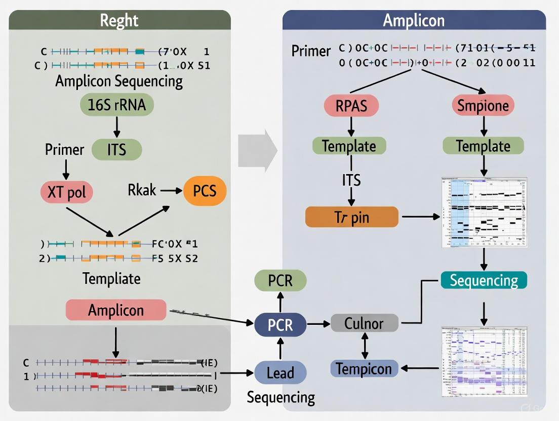
Figure 1: Generalized workflow for 16S rRNA and ITS amplicon sequencing studies, from sample collection through data analysis.
Bioinformatics Analysis Pipelines
Sequence Processing and Clustering
The analysis of amplicon sequencing data begins with quality control and preprocessing of raw sequence reads. This typically involves merging paired-end reads (when using Illumina platforms), quality filtering to remove low-quality sequences, dereplication (collapsing identical sequences), and removing chimeric sequences—artifactual amplicons formed during PCR from multiple parent sequences [8]. These steps are crucial for reducing technical noise before biological interpretation.
Processed sequences are then grouped into taxonomic units using either Operational Taxonomic Units (OTUs) or Amplicon Sequence Variants (ASVs). OTU clustering groups sequences based on a similarity threshold (traditionally 97%), assuming that sequencing errors and minor variations can be collapsed into a single unit [3] [8]. In contrast, ASV methods (also called zOTUs or ESVs) employ denoising algorithms to distinguish biological sequences from sequencing errors, resulting in units that differ by as little as a single nucleotide [3] [8]. ASV approaches (e.g., DADA2, Deblur) generally provide higher resolution and greater reproducibility across studies, while OTU methods (e.g., UPARSE, mothur) may be more robust to sequencing errors in some contexts [8].
Taxonomic Assignment and Diversity Analysis
Taxonomic classification assigns biological identities to OTUs or ASVs by comparing them to reference databases of known microbial sequences. Commonly used databases include GreenGenes (GG), Silva, the Ribosomal Database Project (RDP), and specialized databases for particular environments [3]. The choice of database significantly influences results, as variations in nomenclature, taxonomy, and sequence coverage can lead to different taxonomic assignments for the same sequence [3].
Downstream analysis typically includes measures of alpha diversity (within-sample diversity) and beta diversity (between-sample diversity). Alpha diversity metrics (e.g., Chao1, Simpson index) provide insights into community richness and evenness, while beta diversity measures (e.g., Bray-Curtis dissimilarity, UniFrac distance) enable comparison of community structures across different samples or experimental conditions [8]. These analyses form the basis for identifying statistically significant differences in microbial communities between experimental groups—a key objective in many microbiome studies.
Figure 2: Bioinformatic processing pipeline for 16S rRNA and ITS amplicon sequencing data.
Applications Across Research Fields
Medical and Pharmaceutical Applications
In medical research, 16S rRNA and ITS amplicon sequencing have revolutionized our understanding of the human microbiome's role in health and disease. These approaches have been used to investigate microbiome associations with metabolic diseases, digestive disorders, autoimmune conditions, neurological diseases, and various cancers [9] [1]. The high sensitivity of these methods enables detection of low-abundance pathogens or dysbiotic communities that may contribute to disease pathogenesis.
In drug development, microbiome analysis provides insights into how pharmaceutical interventions alter microbial communities, potentially explaining drug efficacy or side effects. Additionally, the highly individualized nature of human microbiomes has prompted investigation into microbial fingerprints for forensic identification, where an individual's unique microbial signature can be traced from skin, oral, or gut samples [9]. Skin microbiome analysis, for instance, has demonstrated up to 100% classification accuracy for matching samples to specific individuals [9].
Agricultural, Environmental, and Industrial Applications
Beyond human health, targeted amplicon sequencing finds extensive applications in agricultural science, where it is used to study microbial interactions in the rhizosphere, the effects of agricultural practices on soil health, and plant-microbe relationships that influence crop productivity [1]. Understanding these microbial dynamics enables development of sustainable farming practices and microbiome-based solutions for plant health.
In environmental studies, these methods facilitate characterization of microbial communities in diverse habitats—from polluted ecosystems to extreme environments—providing insights into microbial adaptations and ecosystem functioning [1]. Industrial applications include monitoring bioremediation processes, optimizing wastewater treatment systems, and developing bioenergy solutions through identification of functional microbial strains [1]. In each context, the targeted approach provides a cost-effective means to survey microbial community structure and dynamics at scale.
The Scientist's Toolkit: Essential Research Reagents and Materials
Table 3: Key Research Reagent Solutions for 16S/ITS Amplicon Sequencing
| Reagent/Material | Function | Considerations |
|---|---|---|
| Preservation Buffers (e.g., RLT Plus with DTT) | Stabilize nucleic acids during sample storage | RNA stabilizers needed for RNA-based approaches [6] |
| DNA/RNA Extraction Kits (e.g., AllPrep DNA/RNA/miRNA Kit) | Co-purification of DNA and RNA from same sample | Enables parallel DNA- and RNA-based analysis [6] |
| Barcoded PCR Primers | Amplification of target regions with sample indexes | Design affects taxonomic coverage and bias [3] [7] |
| High-Fidelity DNA Polymerase | Accurate amplification with minimal errors | Reduces PCR-derived sequence artifacts |
| PNA Clamps | Suppress host DNA amplification | Critical for low-biomass or host-contaminated samples [7] |
| Positive Control Standards (e.g., ZymoBIOMICS Microbial Community Standard) | Monitor technical performance | Should mimic sample complexity [6] |
| Size Selection Beads | Cleanup and normalization of amplicon libraries | Affect size distribution and remove primer dimers |
| Sequencing Kits (Platform-specific) | Generate sequence data | Read length and error profiles vary by platform [5] [1] |
Methodological Variations and Emerging Approaches
DNA-based vs. RNA-based Approaches
Most amplicon sequencing studies utilize DNA-based approaches, which reflect the total microbial community (including dormant cells and free DNA) present in a sample. However, RNA-based 16S rRNA sequencing is emerging as a complementary approach that specifically targets the active microbiota by reverse transcribing and sequencing rRNA molecules [6]. Since ribosomal RNA is more abundant than rRNA genes in metabolically active cells (e.g., E. coli contains ~25,000 ribosomes per cell), RNA-based approaches offer significantly higher sensitivity, particularly for low-biomass samples [6].
Comparative studies have demonstrated that RNA-based analysis typically reveals higher microbial diversity, with significant differences in alpha and beta diversity metrics compared to DNA-based approaches [6]. However, both methods have biases: DNA-based analysis is influenced by varying rRNA gene copy numbers (1-21 per genome), while RNA-based analysis is affected by differences in ribosome content per cell, which varies with growth rate and cell size [6]. A combined DNA-RNA approach provides the most comprehensive view of microbial communities, distinguishing between present and active members.
Technological Platforms and Their Applications
The evolution of sequencing technologies has dramatically expanded options for amplicon sequencing. Second-generation platforms (e.g., Illumina MiSeq/HiSeq) offer high accuracy and throughput for short reads (up to 600 bp), typically targeting one to three variable regions [3]. Third-generation platforms (e.g., PacBio, Oxford Nanopore) enable full-length 16S rRNA gene sequencing (~1500 bp), providing superior taxonomic resolution to the species and strain level [5].
Full-length sequencing reveals that many bacterial genomes contain multiple polymorphic copies of the 16S rRNA gene that vary slightly in sequence [5]. These intragenomic copy variants have traditionally been collapsed by short-read approaches but can be resolved with long-read technologies, potentially providing additional strain-level discrimination [5]. However, long-read technologies historically had higher error rates, though recent improvements in circular consensus sequencing (CCS) have substantially enhanced accuracy [5]. The choice of platform therefore represents a trade-off between read length, accuracy, throughput, and cost that must be optimized for each research question.
16S rRNA and ITS amplicon sequencing represent powerful, targeted approaches for profiling microbial communities across diverse research contexts. The method's strength lies in its ability to provide comprehensive taxonomic characterization of complex samples in a cost-effective, high-throughput manner. As sequencing technologies continue to evolve—particularly with the emergence of accurate long-read platforms—the taxonomic resolution achievable through these approaches will continue to improve, potentially enabling reliable discrimination at the species and strain level.
Critical considerations for robust experimental design include appropriate selection of variable regions, careful sample handling to preserve community integrity, and implementation of bioinformatic pipelines that minimize technical artifacts while maximizing biological information. For certain applications, emerging variations such as RNA-based sequencing or full-length amplicon approaches may provide valuable complementary insights. As these methodologies become increasingly sophisticated and accessible, they will continue to drive discoveries in microbial ecology, host-microbe interactions, and the diverse roles of microorganisms in health, disease, and ecosystem functioning.
The 16S ribosomal RNA (rRNA) gene is a cornerstone of microbial ecology and serves as the universal genetic barcode for identifying and classifying Bacteria and Archaea [10]. This gene, approximately 1500 base pairs (bp) in length, contains a unique combination of evolutionarily conserved regions and nine hypervariable regions (V1-V9) that provide distinct taxonomic signatures [11] [10]. The conserved regions enable the design of universal polymerase chain reaction (PCR) primers that can amplify this gene from virtually all prokaryotic organisms, while the variable regions contain sufficient sequence diversity to differentiate between microbial taxa at various phylogenetic levels, from domain to species [12].
The utility of the 16S rRNA gene extends beyond mere identification. Its application has revolutionized our understanding of microbial communities in diverse environments, from the human gut to extreme ecosystems. Through targeted amplicon sequencing, researchers can now characterize complex microbial populations without the limitations of culturing, revealing the tremendous diversity of microbial life that was previously undetectable using traditional microbiological methods [10]. The resulting data provide insights into microbial community structure, diversity, dynamics, and ecological functions, making 16S rRNA gene sequencing an indispensable tool in modern microbiology.
Molecular Foundations and Primer Design
Genetic Structure and Phylogenetic Significance
The 16S rRNA gene forms an integral component of the prokaryotic 30S ribosomal subunit, playing a critical role in protein synthesis by facilitating the initiation of mRNA translation and ensuring proper codon-anticodon pairing [13]. The gene's remarkable suitability as a phylogenetic marker stems from its functional constancy, universal distribution across prokaryotes, and appropriate evolutionary clock properties, with variable regions evolving at different rates that provide resolution at different taxonomic levels [13] [12].
The central pseudoknot structure, formed by nucleotides 17-19 pairing with nucleotides 916-918, represents a particularly conserved and functionally essential region of the 16S rRNA molecule [13]. This structural element is crucial for translational initiation and exhibits high susceptibility to point mutations, making it a critical consideration in primer design and functional studies [13]. The conservation of this and other functional domains ensures that the 16S rRNA gene maintains its essential cellular function while accumulating neutral mutations in non-critical regions that provide phylogenetic information.
Primer Design Strategies and Considerations
The design of PCR primers for 16S rRNA gene amplification represents a critical methodological step that directly influences experimental outcomes. Effective primer design must balance multiple competing objectives: maximizing coverage (the fraction of bacterial 16S sequences successfully targeted), optimizing efficiency (the ability to amplify target sequences specifically and robustly), and minimizing primer matching-bias (differential amplification of certain taxa over others) [14].
Computational approaches like the Multi-Objective Primer Optimization for 16S experiments (mopo16S) algorithm have been developed to systematically evaluate and optimize primer sets based on these criteria [14]. These methods employ multi-objective optimization that simultaneously considers thermodynamic properties (melting temperature, GC-content), structural characteristics (3'-end stability, secondary structure formation), and taxonomic coverage against comprehensive 16S rRNA reference databases [14]. The development of degenerate primers—mixtures of oligonucleotides with variations at specific positions—has further enhanced the ability to target diverse microbial taxa, though these introduce challenges in reproducible synthesis and potential amplification biases [14].
Table 1: Key Considerations for 16S rRNA Primer Design
| Parameter | Optimal Range | Impact on Performance |
|---|---|---|
| Melting Temperature (Tm) | 52°C or higher | Primer binding efficiency; specificity of amplification |
| GC Content | 40-70% | Specificity and stability of primer-template binding |
| 3'-End Stability | Avoid poly-A/T tracts | Prevention of non-specific amplification |
| Primer Length | 18-25 bp | Balance between specificity and coverage |
| Degenerate Positions | Minimize when possible | Reduced synthesis reproducibility and potential bias |
Recent advances in primer design have addressed previously overlooked mismatches at critical positions. For example, the common universal primers Bac8f and UN1541r overlap variable sites at positions 19 and 1527, which can introduce mutations during amplification, particularly problematic at position 19 due to its involvement in the central pseudoknot [13]. New primer sets such as Bac1f and UN1542r have been designed to avoid these mismatch sites, improving amplification accuracy [13].
Experimental Approaches and Sequencing Platforms
Short-Read versus Long-Read Sequencing
The selection of sequencing platform represents a fundamental methodological choice that governs the scope and resolution of 16S rRNA gene analysis. Short-read sequencing platforms, particularly Illumina systems, have traditionally dominated 16S rRNA sequencing due to their high throughput, low per-base cost, and well-established analytical pipelines [11] [10]. However, these platforms are limited by read length constraints, typically targeting only 1-3 variable regions (such as V3-V4 or V4-V5) in a single experiment, which restricts taxonomic resolution, often to the genus level [11] [15].
In contrast, long-read sequencing technologies offered by Oxford Nanopore Technologies (ONT) and Pacific Biosciences (PacBio) enable full-length 16S rRNA gene sequencing (~1500 bp) or even entire ribosomal RNA operon (RRN) sequencing (~4500 bp), which spans the 16S-ITS-23S genomic region [16] [15]. This comprehensive approach captures all variable regions and provides substantially improved phylogenetic resolution, frequently enabling species-level and sometimes strain-level discrimination [15]. The advancement of these platforms, particularly with ONT's Q20+ chemistry and PacBio's HiFi sequencing, has addressed earlier limitations in accuracy, making long-read approaches increasingly viable for high-resolution microbial profiling [15].
Table 2: Comparison of 16S rRNA Sequencing Approaches
| Platform | Read Length | Target Region | Taxonomic Resolution | Key Applications |
|---|---|---|---|---|
| Illumina MiSeq | 2×300 bp | Single or dual variable regions (e.g., V3-V4) | Genus-level | High-throughput community profiling |
| xGen Amplicon Panel | Multiple discontinuous regions | All 9 variable regions (separate amplicons) | Species-level with multi-region approach | Species-level identification from short reads |
| PacBio HiFi | Full-length 16S (~1500 bp) | Entire 16S rRNA gene | Species-level | High-accuracy full-length sequencing |
| Oxford Nanopore | Full-length 16S or RRN | Complete 16S or 16S-ITS-23S operon | Species to strain-level | Real-time sequencing; portable analysis |
Multi-Variable Region Sequencing with Short-Read Platforms
Innovative approaches have been developed to enhance taxonomic resolution while maintaining the benefits of short-read sequencing. The xGen 16S Amplicon Panel v2 utilizes multiple primer pairs to generate amplicons covering all nine variable regions of the 16S rRNA gene, which are sequenced concurrently on Illumina platforms [11]. When processed through specialized bioinformatics pipelines like Swift Normalase Amplicon Panels APP for Python 3 (SNAPP-py3), this method achieves species-level resolution typically associated with long-read approaches while leveraging the cost-effectiveness and throughput of Illumina sequencing [11].
This multi-region approach addresses the fundamental limitation of single-region sequencing by capturing complementary taxonomic information from different variable regions, as each region possesses different discriminatory power for various bacterial taxa [11]. The method has demonstrated high reproducibility in technical replicates and accurate species-level identification in mock communities, with observed relative abundances closely matching theoretical expectations [11].
Detailed Experimental Protocols
Sample Collection and DNA Extraction
The initial steps of sample collection and nucleic acid extraction critically influence downstream results in 16S rRNA gene sequencing. Collection methods must be tailored to the sample type—whether stool, rectal swabs, tissue, or environmental samples—as different collection approaches can yield substantially different microbial profiles even when sampling the same source [11] [17]. For example, concurrent stool and rectal swab samples from the same infants show significant differences in microbial composition, highlighting the importance of consistent methodology throughout a study [11].
DNA extraction should be optimized for the specific sample type to maximize yield while preserving accurate community representation. Key considerations include cell lysis efficiency across different bacterial taxa (Gram-positive versus Gram-negative), inhibition removal, and minimization of DNA shearing. The inclusion of mock community controls containing known quantities of specific bacterial species is essential for evaluating extraction efficiency and identifying technical biases introduced during this process [11] [17].
Library Preparation and Sequencing
Short-Red Multi-Variable Region Protocol (xGen 16S Amplicon Panel)
The xGen 16S Amplicon Panel v2 enables comprehensive profiling of all nine variable regions through the following workflow [11]:
DNA Quality Assessment: Verify DNA quantity and quality using fluorometric methods (e.g., Qubit) and ensure integrity through electrophoretic analysis.
Multiplex PCR Amplification: Utilize the panel's primer mixture to simultaneously amplify all variable regions of the 16S rRNA gene in a single, multiplexed reaction.
Library Construction: Process amplicons through indexing PCR to add sample-specific barcodes and sequencing adapters compatible with Illumina platforms.
Library Normalization and Pooling: Quantify individual libraries, normalize to equimolar concentrations, and combine into a single sequencing pool.
Sequencing: Load the pooled library onto an Illumina MiSeq or similar instrument using appropriate read length (e.g., 2×300 bp) to ensure sufficient overlap for paired-end assembly.
This protocol is particularly valuable when species-level resolution is required but access to long-read sequencing is limited, providing a compromise between information content and platform accessibility [11].
Full-Length 16S and RRN Sequencing (Oxford Nanopore Protocol)
The Oxford Nanopore Microbial Amplicon Barcoding Kit (SQK-MAB114.24) provides a workflow for full-length 16S or ITS sequencing [16]:
PCR Amplification: Amplify the full-length 16S rRNA gene using inclusive primers designed for broad taxonomic coverage. Reaction conditions: 10 ng gDNA template, LongAmp Hot Start Taq 2X Master Mix, 16S-specific primers, with thermal cycling parameters according to manufacturer specifications.
Amplicon Barcoding: Attach unique barcodes to individual amplicon samples using a 15-minute barcoding reaction, enabling multiplexing of up to 24 samples.
Pooling and Clean-up: Combine barcoded samples and purify using bead-based clean-up to remove primers, dimers, and other contaminants.
Adapter Ligation: Rapidly attach sequencing adapters (5 minutes) without additional PCR amplification, preserving the integrity of full-length amplicons.
Priming and Loading: Prepare the flow cell with priming buffer and load the adapted library for sequencing.
Sequencing and Real-time Analysis: Initiate sequencing runs through MinKNOW software, with optional real-time analysis through EPI2ME 16S workflow for immediate taxonomic classification [16].
This fragmentation-free workflow preserves full-length amplicons, enabling complete coverage of the 16S rRNA gene and maximizing phylogenetic resolution [16].
Bioinformatics Analysis Pipelines
The analysis of 16S rRNA gene sequencing data requires specialized bioinformatics tools to transform raw sequence data into biological insights. Two established platforms, QIIME (Quantitative Insights Into Microbial Ecology) and mothur, provide comprehensive pipelines for processing 16S rRNA amplicon data [18]. These toolsets incorporate quality filtering, chimera detection, sequence clustering, taxonomic classification, and diversity analysis in reproducible workflows.
For users seeking more accessible interfaces, the Galaxy mothur Toolset (GmT) provides a user-friendly web interface for the complete suite of mothur tools, enabling researchers without command-line expertise to perform sophisticated analyses [19]. The standard GmT workflow includes [19]:
- Read Processing: Pair-end read merging (make.contigs) and quality trimming (trim.seqs)
- Alignment and Filtering: Alignment to reference databases (align.seqs) and sequence screening (screen.seqs)
- Chimera Removal: Identification and removal of chimeric sequences (chimera.uchime)
- Taxonomic Classification: Bayesian classification against reference databases (classify.seqs)
- OTU Clustering: Distance calculation (dist.seqs) and OTU clustering at 97% similarity (cluster)
- Diversity Analysis: α- and β-diversity calculations and visualization
The emergence of long-read sequencing has necessitated the development of specialized classification approaches for full-length 16S and RRN data. The Minimap2 classifier in combination with comprehensive databases like GROND has demonstrated superior performance for species-level classification of RRN sequencing data, outperforming traditional OTU-clustering methods [15].
16S rRNA Gene Analysis Workflow: From Sample to Interpretation
Essential Research Reagents and Tools
Table 3: Essential Research Reagents and Computational Tools for 16S rRNA Gene Analysis
| Category | Specific Product/Tool | Function/Application |
|---|---|---|
| Wet Lab Kits | xGen 16S Amplicon Panel v2 | Amplification of all 9 variable regions for Illumina sequencing |
| Microbial Amplicon Barcoding Kit (ONT) | Full-length 16S or ITS sequencing on Nanopore platforms | |
| ZymoBIOMICS Microbial Standards | Mock community controls for quality validation | |
| Bioinformatics Tools | QIIME 2 | Comprehensive pipeline for 16S rRNA data analysis |
| mothur | Open-source platform for microbial community analysis | |
| Galaxy mothur Toolset (GmT) | Web-based interface for mothur tools | |
| Minimap2 | Alignment tool for long-read 16S and RRN data | |
| Reference Databases | SILVA | Curated database of aligned ribosomal RNA sequences |
| GreenGenes | 16S rRNA gene database and taxonomy | |
| GROND | Database for ribosomal RNA operon analysis | |
| RDP (Ribosomal Database Project) | Annotated database of rRNA sequences |
Applications and Best Practices
Applications in Microbial Research
The applications of 16S rRNA gene sequencing span diverse research areas, from clinical microbiology to environmental science. In human microbiome studies, this approach has revealed microbial dysbiosis associated with chronic conditions such as chronic rhinosinusitis (CRS), where decreased microbial diversity and altered abundance of specific taxa correlate with disease severity and clinical outcomes [12]. In agricultural research, 16S rRNA profiling has characterized poultry gastrointestinal microbiota and its relationship to host health, nutrition, and growth performance [17].
The technology continues to evolve with emerging applications in forensic microbiology, bioremediation monitoring, food safety, and built environment analysis. The expanding utilization of this method across disciplines underscores its fundamental importance in understanding microbial systems in virtually every environment on Earth.
Standardization and Reproducibility Considerations
The proliferation of 16S rRNA gene sequencing applications has revealed significant challenges in methodological standardization and reproducibility. Variations in DNA extraction protocols, primer selection, sequencing platforms, and bioinformatic analyses can introduce substantial biases, affecting community structure representation and leading to over- or under-estimation of specific taxa [17]. These methodological differences make cross-study comparisons problematic and highlight the need for standardized protocols within research communities.
Best practices to enhance reproducibility include [11] [17]:
Incorporation of Mock Controls: Routine use of defined microbial communities to quantify technical variability and accuracy.
Detailed Methodological Reporting: Comprehensive documentation of DNA extraction methods, primer sequences, PCR conditions, and bioinformatic parameters.
Platform Validation: Assessment of multiple variable regions or full-length sequencing when possible to overcome region-specific biases.
Data Sharing and Public Archiving: Deposition of raw sequence data and associated metadata in public repositories to enable reanalysis and comparison.
Database Consistency: Use of consistent, curated reference databases with version control to ensure comparable taxonomic classifications.
The development of field-specific guidelines for 16S rRNA gene sequencing, encompassing sample collection through data deposition, represents an ongoing effort to improve reliability and comparability across microbial community studies [17].
The 16S rRNA gene remains an indispensable tool for microbial identification and community analysis, continuing to provide fundamental insights into the diversity, ecology, and function of prokaryotic communities across diverse environments. Advances in sequencing technologies, particularly the emergence of long-read platforms and multi-region amplification approaches, have enhanced the resolution and accuracy of 16S rRNA-based studies, enabling species-level discrimination that was previously challenging with short-read methods.
As the field continues to evolve, the integration of 16S rRNA gene sequencing with other 'omics approaches—including metagenomics, metatranscriptomics, and metabolomics—will provide more comprehensive understanding of microbial community structure and function. Similarly, the development of standardized protocols and reference materials will strengthen the reproducibility and comparability of findings across studies. Through these continued methodological refinements and applications, 16S rRNA gene sequencing will maintain its central role in advancing our understanding of the microbial world that shapes human health, ecosystem function, and global biogeochemical cycles.
The Internal Transcribed Spacer (ITS) region of the ribosomal RNA (rRNA) gene cluster has been established as the official primary DNA barcode for fungi, providing a powerful tool for mycologists, ecologists, and drug development professionals engaged in microbial community analysis [10] [20]. This non-coding region, characterized by significant sequence variability and flanked by highly conserved genes, enables precise taxonomic classification and has become the cornerstone of modern fungal diversity studies using amplicon sequencing technologies [21] [22].
The adoption of the ITS region as the universal fungal barcode stems from several key advantages: its multicopy nature within the fungal genome, which facilitates amplification from minute quantities of DNA; the presence of conserved regions that allow for the design of broad-range primers; and sufficient sequence variation to discriminate between closely related species across the fungal kingdom [10] [23] [22]. Compared to other genetic markers, the ITS region offers an optimal balance of conservation and variability, making it particularly suitable for phylogenetic studies and environmental sampling where unknown fungal diversity is expected [24] [1].
The ITS Region: Structure and Rationale for Fungal Barcoding
Molecular Architecture
The ITS region is located within the rRNA gene cluster and consists of two variable spacers:
- ITS1: Located between the 18S (small subunit) and 5.8S rRNA genes, typically ranging from 150-400 bp in length [24]
- ITS2: Situated between the 5.8S and 28S (large subunit) rRNA genes, with a similar length range to ITS1 [21]
- Flanking regions: The ITS region is bounded by the 18S, 5.8S, and 28S rRNA genes, which contain conserved sequences ideal for primer binding [21] [1]
The complete ITS region (including the 5.8S gene) typically spans 500-750 base pairs, though this length can vary considerably across fungal taxa [21]. This variability in length and sequence composition provides the phylogenetic signal necessary for distinguishing between species.
Comparative Advantages Over Alternative Markers
While other genetic regions such as RPB1, RPB2, β-tubulin, and TEF1α (the secondary fungal barcode) may offer superior discrimination for specific taxonomic groups, the ITS region remains the most comprehensively utilized marker for fungal identification [24]. Key comparative advantages include:
- Amplification success: Higher amplification rates across diverse fungal taxa compared to protein-coding genes [24]
- Database coverage: Substantially more reference sequences in public databases than any other fungal marker [24]
- Taxonomic resolution: Generally provides species-level identification for most fungi, though resolution varies among genera [24] [20]
The ITS region's limitations are most apparent in certain ubiquitous genera such as Aspergillus and Penicillium, where interspecific variation may be insufficient for reliable discrimination [24] [20]. In such cases, supplemental markers may be required for definitive identification.
Experimental Performance and Comparative Analysis
Assessment of ITS1 versus ITS2 Subregions
The length of the complete ITS region (500-700 bp) often exceeds the optimal read length of widely used Illumina platforms, necessitating targeted sequencing of either the ITS1 or ITS2 subregion [24]. Research using defined mock communities has yielded important insights into the comparative performance of these subregions:
Table 1: Performance comparison of ITS1 and ITS2 subregions based on defined mock community analysis
| Parameter | ITS1 | ITS2 | Experimental Context |
|---|---|---|---|
| Precision | Lower | Slightly better | Illumina sequencing of 37 defined mock communities [24] |
| Recall | Comparable | Comparable | Illumina sequencing of 37 defined mock communities [24] |
| Amplicon Length | 150-400 bp | 150-400 bp | Varies by taxonomic group [24] |
| Primer Universality | Fewer universal primer sites | More universal primer sites | Affects amplification success across diverse taxa [24] |
| Diversity Estimation | May overestimate diversity | More conservative estimates | Due to higher variability in ITS1 [24] |
| Database Representation | Variable by taxonomic group | Variable by taxonomic group | Affects classification accuracy [24] |
The choice between ITS1 and ITS2 involves trade-offs that must be considered in experimental design. While ITS2 typically provides slightly better precision with comparable recall, the optimal subregion may depend on the specific fungal taxa being investigated and the reference databases available for classification [24].
Bioinformatics and Database Considerations
Classification accuracy in ITS sequencing depends critically on bioinformatics tools and reference database selection:
Table 2: Impact of bioinformatics methods and databases on classification accuracy
| Factor | Options | Performance Considerations | Experimental Evidence |
|---|---|---|---|
| Classification Algorithm | BLAST | Better performance but may require expert curation | Mock community evaluation [24] |
| mothur (Bayesian) | Better performance in automated workflow | Mock community evaluation [24] | |
| Reference Database | UNITE | Widely adopted, species hypotheses | Variable performance depending on taxa [24] |
| BCCM/IHEM | Specialized collection, better for medical fungi | Outperformed UNITE in mock community study [24] | |
| NCBI RTL/ISHAM | Curated databases for specific applications | Important for pathogenic fungi [24] | |
| Taxonomic Level | Species level | Challenging for some genera (e.g., Aspergillus, Penicillium) | Lower precision compared to genus level [24] |
| Genus level | Generally reliable classification | Good precision and recall [24] | |
| Intermediate levels | May present adequate alternatives | Species complex or section level [24] |
Recent research demonstrates that classification performance varies considerably depending on all considered variables, with 56-100% of species correctly assigned across different experimental setups [24]. The reference database employed has a marked effect, with specialized databases such as BCCM/IHEM sometimes outperforming more general databases like UNITE, likely due to differences in sequence curation and taxonomic coverage relevant to specific research questions [24].
Wet Laboratory Protocols
Sample Collection and DNA Extraction
Environmental Sample Collection:
- Air samples: Collect using cyclonic samplers (e.g., NIOSH BC251) at 2-15 L/min onto 0.8 μm mixed cellulose ester filters [22]
- Dust samples: Composite collections from vacuum bags or sieved dust (300-mesh) from carpets and floors [22]
- Clinical specimens: Swabs, tissue biopsies, or bodily fluids collected in sterile containers
- Soil/water: Collection of representative samples using sterile corers or filtration systems
DNA Extraction Protocol:
- Mechanical disruption: Process samples with glass beads (212-300 μm) in a bead beater for 15-30 seconds at high speed [22]
- Lysis: Add commercial lysis buffer (e.g., High Pure PCR Template Kit) and incubate according to manufacturer specifications
- DNA purification: Bind DNA to silica columns, wash with appropriate buffers, and elute in 50-100 μL elution buffer [22]
- Quality assessment: Quantify DNA using fluorometric methods and verify quality via spectrophotometry (A260/A280 ratio ≥1.8)
PCR Amplification and Library Preparation
Primer Selection:
- ITS1-F/ITS2: For ITS1 region amplification (~300 bp) [25]
- ITS3/ITS4: For ITS2 region amplification (~400 bp) [25]
- Full-ITS primers: For long-read sequencing platforms (PacBio, Oxford Nanopore)
Amplification Protocol:
- Reaction setup:
- 2X PCR Master Mix: 25 μL
- Forward primer (10 μM): 2.5 μL
- Reverse primer (10 μM): 2.5 μL
- DNA template: 2-10 ng
- Nuclease-free water to 50 μL
Thermal cycling conditions:
- Initial denaturation: 95°C for 3-5 minutes
- 25-35 cycles of:
- Denaturation: 95°C for 30 seconds
- Annealing: 50-55°C for 30-45 seconds
- Extension: 72°C for 60-90 seconds
- Final extension: 72°C for 5-10 minutes
Library preparation:
- Clean amplified products using magnetic beads
- Attach platform-specific adapters and barcodes
- Validate library quality using bioanalyzer or tape station
Bioinformatics Analysis Workflow
Data Processing and Taxonomic Classification
Quality Control and Denoising:
- Raw read processing:
- Demultiplex samples based on barcodes
- Trim primers and adapters using tools like cutadapt [25]
- Quality filtering based on Q-scores (typically Q≥20)
Denoising approaches:
- DADA2: For Illumina data to resolve amplicon sequence variants (ASVs) [25]
- Deblur: For single-end Illumina data with quality trimming
- UNOISE: For denoising and chimera removal
Sequence clustering:
Taxonomic Classification:
- Reference-based assignment:
- Align sequences to curated databases (UNITE, BCCM/IHEM) using BLAST, Naive Bayes, or alignment tools [24]
- Consider both percent identity and query coverage thresholds
- Confidence assessment:
- Apply bootstrap thresholds (typically ≥80%) for reliable assignments
- Consider taxonomic hierarchies from species to phylum level
Diversity and Community Analysis
Alpha Diversity (within-sample diversity):
- Richness estimators: Chao1, ACE, observed OTUs/ASVs
- Diversity indices: Shannon, Simpson, Inverse Simpson
- Evenness: Pielou's evenness, Simpson's evenness
Beta Diversity (between-sample diversity):
- Distance metrics: Bray-Curtis, Jaccard, Unweighted/Weighted UniFrac
- Ordination methods: PCoA, NMDS, CCA
- Statistical testing: PERMANOVA, ANOSIM, Mantel test
Differential Abundance Analysis:
- Statistical tests: DESeq2, edgeR, LEfSe, METASTATS
- Multivariate methods: RDA, CCA for environmental correlations
The Scientist's Toolkit: Essential Research Reagents and Materials
Table 3: Essential research reagents and materials for fungal ITS analysis
| Category | Specific Product/Kit | Application Purpose | Key Considerations |
|---|---|---|---|
| DNA Extraction | High Pure PCR Template Kit (Roche) | Efficient DNA extraction from complex samples | Optimal for air and dust samples [22] |
| DNeasy PowerSoil Kit (Qiagen) | DNA extraction from soil and environmental samples | Effective for difficult-to-lyse fungi | |
| PCR Amplification | ITS1-F/ITS2 primers | Amplification of ITS1 subregion | Fragment size ~300 bp [25] |
| ITS3/ITS4 primers | Amplification of ITS2 subregion | Fragment size ~400 bp [25] | |
| 5.8S-Fun/ITS4-Fun primers | Full ITS amplification for specific applications | Amplicon range: 267-511 bp [25] | |
| Library Preparation | Illumina DNA Prep | Library construction for Illumina platforms | Integrated workflow for amplicon sequencing [10] |
| SQK-16S024 kit (Oxford Nanopore) | Full-length ITS sequencing | Enables long-read ITS analysis [15] | |
| Quality Control | Agilent Bioanalyzer | Library quality assessment | Determines fragment size distribution |
| Qubit Fluorometer | DNA quantification | More accurate than spectrophotometry for low concentrations | |
| Bioinformatics | QIIME2 platform | End-to-end analysis of ITS data | Extensive plugin ecosystem [25] |
| mothur pipeline | Alternative analysis workflow | Well-established for microbial communities [24] | |
| UNITE database | Primary reference for taxonomic assignment | Species hypotheses approach [24] [25] | |
| BCCM/IHEM database | Specialized database for medical fungi | Enhanced performance for clinical isolates [24] |
Applications in Research and Drug Development
Environmental Mycology
ITS-based metabarcoding has revolutionized environmental mycology by providing culture-independent characterization of fungal communities:
- Indoor mycology: Identification of diverse Ascomycota and Basidiomycota communities in homes of asthmatic children, revealing previously overlooked taxa with potential health implications [22]
- Agricultural systems: Analysis of rhizosphere fungi and their responses to agricultural practices, with potential applications in crop protection and soil health assessment
- Biogeographic studies: Investigation of fungal distribution patterns across environmental gradients and ecosystem types
Clinical and Pharmaceutical Applications
The precision of ITS sequencing enables critical applications in clinical diagnostics and drug discovery:
- Clinical mycology: Species-level identification of pathogens in otomycosis cases, revealing Aspergillus as the dominant pathogen and Malassezia as prevalent in healthy ears [21]
- Drug discovery: Identification of novel fungal species from unique environments as potential sources of bioactive compounds
- Pharmaceutical quality control: Detection of fungal contaminants in manufacturing environments and finished products
Methodological Considerations and Limitations
Despite its utility, researchers must acknowledge several methodological considerations:
- Intragenomic variation: Approximately 65% of multi-copy fungal genomes contain ITS sequence variation, which can affect diversity estimates and taxonomic assignments [23]
- Database inaccuracies: Up to 20% of public repository sequences may be incorrectly annotated, emphasizing the need for curated databases [24]
- Technical biases: DNA extraction efficiency, primer selection, and PCR conditions can all influence community representation [24] [22]
The ITS region remains the gold standard for fungal identification and diversity assessment, offering unparalleled taxonomic resolution across most fungal groups. While challenges persist in species-level discrimination for certain genera and in managing technical artifacts, ongoing refinements in sequencing technologies, reference databases, and bioinformatics pipelines continue to enhance its utility. For researchers and drug development professionals, ITS-based approaches provide a powerful framework for exploring fungal communities in diverse contexts, from environmental ecosystems to clinical settings, with important implications for ecological understanding, public health, and biotechnological innovation.
Advantages and Inherent Limitations of Culture-Free Microbial Profiling
Culture-free microbial profiling, primarily through 16S rRNA and ITS amplicon sequencing, has revolutionized microbial community analysis by enabling comprehensive biodiversity assessment beyond the constraints of cultivability. These methods provide unprecedented insights into microbial community composition, dynamics, and functional potential across diverse environments from human health to industrial applications. However, inherent technical and biological limitations—including primer bias, variable gene copy numbers, inability to distinguish viable from non-viable cells, and analytical pipeline dependencies—significantly impact data interpretation. This application note delineates the advantages and limitations of culture-free profiling methodologies within 16S rRNA and ITS research frameworks, providing structured experimental protocols, quantitative performance comparisons, and standardized workflows to enhance research reproducibility and analytical accuracy for scientists and drug development professionals.
Traditional microbial characterization relying on laboratory cultivation has historically limited our understanding of microbial diversity, as an estimated 99% of microorganisms cannot be cultured under standard laboratory conditions [26]. Culture-free microbial profiling, utilizing targeted amplicon sequencing of phylogenetic marker genes such as the 16S ribosomal RNA (rRNA) gene for bacteria and archaea and the Internal Transcribed Spacer (ITS) region for fungi, has fundamentally transformed microbial ecology and diagnostics. This approach enables the precise identification and relative quantification of microbial taxa directly from complex samples without cultivation bias [27] [28].
The power of these methods lies in their ability to provide high-resolution community analysis from diverse sample types, including human tissues, environmental samples, and industrial products. By targeting conserved yet variable genetic regions, researchers can characterize microbiomes at various taxonomic levels, exploring community shifts in response to disease, environmental changes, or therapeutic interventions [29] [28]. Despite their transformative impact, the techniques carry inherent limitations that must be acknowledged and mitigated to ensure biologically accurate interpretations. This application note details the balanced landscape of culture-free microbial profiling, providing a framework for its rigorous application in research and drug development.
Advantages of Culture-Free Microbial Profiling
Comprehensive Community Analysis
Unlike culture-dependent methods that selectively isolate microorganisms based on their growth requirements, culture-free profiling captures the entire microbial community present in a sample.
- Identification of Unculturable Taxa: Advanced Microbial Profiling (AMP) reveals organisms that are difficult or impossible to culture in the lab, providing a more complete picture of microbial diversity [26].
- Detection of Injured and Viable-but-Non-Culturable (VBNC) Cells: The method identifies both healthy and metabolically compromised microbial cells that would otherwise escape detection through traditional culturing [26].
- High-Throughput Capacity: The technology can analyze dozens of samples simultaneously, generating thousands of microbial marker sequences per sample in a single run, enabling robust statistical analysis and population dynamics studies [26].
Enhanced Sensitivity and Resolution
The sensitivity of culture-free methods significantly surpasses traditional approaches, enabling detection of low-abundance taxa and fine-scale differentiation between closely related organisms.
- Superior Sensitivity: RNA-based 16S rRNA sequencing demonstrates at least a 10-fold higher sensitivity compared to DNA-based approaches, enabling detection of rare taxa in low-biomass samples like the uterine microbiome [6].
- Strain-Level Differentiation: Amplicon Sequence Variant (ASV) methods like DADA2 offer single-nucleotide resolution, providing finer taxonomic precision than traditional Operational Taxonomic Unit (OTU) clustering and enabling tracking of specific bacterial strains within communities [28].
Diagnostic and Predictive Capabilities
Culture-free profiling has demonstrated significant utility in clinical diagnostics by detecting pathogens that evade traditional methods and providing predictive insights into microbial community functions.
- Clinical Pathogen Detection: The MYcrobiota platform confirmed bacterial DNA in 37/37 culture-positive clinical samples and detected potentially relevant bacterial taxa in 2/10 culture-negative samples, demonstrating 95% sensitivity and specificity compared to culture [29].
- Functional Prediction: Tools like Tax4Fun predict functional profiles from 16S rRNA data, linking phylogenetic information to potential metabolic capabilities within microbial communities [30].
- Process Monitoring: In anaerobic digestion, linking microbial community dynamics to operational parameters allows for better process control and stability prediction [30].
Table 1: Quantitative Advantages of Culture-Free vs. Culture-Based Methods
| Parameter | Culture-Free Profiling | Traditional Culturing |
|---|---|---|
| Detection Threshold | 0.01% relative abundance [28] | ≥1% (culture-dependent) |
| Taxonomic Resolution | Species/Strain level (ASV) [28] | Species level (MALDI-TOF) [29] |
| Process Time | 1-3 days [28] | 2-5 days [29] |
| Throughput | Dozens of samples simultaneously [26] | Limited by cultivation space |
| Unculturable Detection | Yes [26] | No |
| Sensitivity in Low Biomass | 10-fold higher for RNA-based [6] | Limited |
Inherent Limitations and Biases
Technical and Methodological Biases
Multiple technical steps in culture-free profiling introduce distortions that may not accurately reflect the original microbial community composition.
- Primer Selection Bias: The choice of primer pairs and amplified variable regions (e.g., V3-V4, V4-V5) significantly influences which taxa are detected and their relative abundances [31] [28]. Different hypervariable regions exhibit varying degrees of conservation and discrimination power.
- DNA Extraction Efficiency: Lysis efficiency varies across microbial taxa due to differences in cell wall structure, potentially underrepresenting difficult-to-lyse organisms like Gram-positive bacteria [6].
- PCR Amplification Bias: During amplification, template-specific variations in PCR efficiencies (PCR competition) and formation of chimeric sequences distort abundance measurements, particularly in polymicrobial samples [29].
- Gene Copy Number Variation: The 16S rRNA gene copy number varies significantly (1-21 copies per genome) across bacterial taxa, leading to overestimation of species with high copy numbers and underestimation of those with low copy numbers when using DNA-based approaches [6].
Biological Limitations
Fundamental biological considerations limit the interpretation of data generated from culture-free profiling approaches.
- Viability Assessment: DNA-based analysis cannot distinguish between live bacteria, dead cells, and free bacterial DNA, potentially leading to false positive results in viability-dependent contexts [29] [6].
- Ribosomal Content Variability: RNA-based approaches are biased by the number of ribosomes per cell, which varies with growth rate, cell size, and metabolic activity, complicating abundance quantification [6].
- Host DNA Contamination: In low-microbial-biomass samples (e.g., BALF, tissue biopsies), host DNA can comprise over 99.99% of total DNA, drastically reducing microbial sequencing depth unless depletion methods are employed [32].
Analytical and Bioinformatics Challenges
The interpretation of sequencing data is heavily dependent on bioinformatics pipelines, which can yield dramatically different biological conclusions.
- Pipeline-Dependent Results: Common analysis tools (QIIME, Mothur, QIIME2) produce significantly different taxonomic compositions from the same environmental dataset, with abundant taxa potentially going undetected depending on the pipeline selected [33].
- Contamination Sensitivity: The techniques are highly susceptible to contamination from laboratory reagents and environments, particularly problematic for low-biomass samples where contaminant DNA can exceed target DNA [29] [32].
- Database Limitations: Incomplete reference databases lead to limited read assignment and substantial gaps in data interpretation, particularly for novel or understudied lineages [30].
Table 2: Systematic Biases in Culture-Free Profiling Methodologies
| Bias Type | Impact on Results | Mitigation Strategies |
|---|---|---|
| Primer Selection | Variable detection of taxa; abundance distortion [31] | Use well-validated primer sets; multiple variable regions |
| Gene Copy Number | Over/under-estimation of taxa abundance [6] | Apply copy number correction algorithms |
| Viability Blindness | Detection of non-viable cells and free DNA [6] | Incorporate propidium monoazide (PMA) treatment |
| Host DNA Contamination | Reduced microbial sequencing depth [32] | Implement host depletion methods (saponin, nucleases) |
| PCR Artifacts | Chimera formation; abundance inaccuracies [29] | Use micelle PCR; internal calibrators; validation |
| Bioinformatic Pipeline | Dramatically different community profiles [33] | Standardize pipeline; mock community validation |
Experimental Protocols
DNA- and RNA-Based 16S rRNA Amplicon Sequencing
This protocol outlines a simultaneous DNA and RNA extraction method followed by 16S rRNA (gene) amplicon sequencing to differentiate between total and active microbial communities [30] [6].
Sample Preparation and Nucleic Acid Extraction:
- Sample Preservation: Immediately freeze samples at -80°C or in liquid nitrogen. For RNA preservation, add 25% glycerol to samples before freezing [32].
- Simultaneous DNA/RNA Extraction: Use the RNA PowerSoil Total RNA Isolation Kit with the RNA PowerSoil DNA Elution Accessory Kit (MoBio Laboratories) for co-extraction [30].
- DNase Treatment: Treat RNA extracts with DNase I Kit for Purified RNA in Solution to remove residual DNA. Validate DNA removal via PCR amplification of the 16S rRNA gene followed by agarose gel electrophoresis [30].
- cDNA Synthesis: Convert RNA to cDNA using the qScriber cDNA Synthesis Kit [30].
- Quality Control: Assess nucleic acid quality and concentration using Nanodrop spectrophotometry and fluorometric methods (e.g., QuantiFluor RNA/DNA Systems) [6].
16S rRNA Gene Amplification and Sequencing:
- Primer Selection: Target the V3-V4 hypervariable region using primers 341F (CCTACGGGNGGCWGCAG) and 785R (GACTACHVGGGTATCTAATCC) for bacterial communities [30].
- PCR Amplification: Perform amplification using Phusion high-fidelity DNA polymerase with the following cycling conditions: initial denaturation at 95°C for 5 min; 25-30 cycles of 95°C for 40 sec, 53°C for 40 sec, 72°C for 60 sec; final elongation at 72°C for 7 min [31].
- Library Preparation and Sequencing: Purify amplicons using Agencourt AMPure XP beads, prepare Illumina-compatible libraries using the Ovation Rapid DR Multiplex System, and sequence on Illumina MiSeq or NovaSeq platforms with 200-250bp paired-end reads [30] [28].
Host DNA Depletion for Low-Biomass Samples
For samples with high host-to-microbe ratios (e.g., BALF, tissue biopsies), implement host DNA depletion to increase microbial sequencing depth [32].
Pre-extraction Methods (Select one approach):
- Saponin Lysis with Nuclease Digestion (S_ase):
- Treat sample with 0.025% saponin to lyse mammalian cells
- Follow with nuclease digestion to degrade released host DNA
- Centrifuge to pellet intact microbial cells
- Proceed with DNA extraction from pellet [32]
- Filter-based Method with Nuclease Digestion (F_ase):
- Filter sample through 10μm filter to separate microbial from host cells
- Treat filtrate with nuclease to digest cell-free DNA
- Collect microbial cells via centrifugation
- Proceed with DNA extraction [32]
Quality Control:
- Quantify host DNA depletion efficiency via qPCR targeting human-specific genes (e.g., β-actin)
- Monitor bacterial DNA retention using 16S rRNA gene qPCR [32]
Figure 1: Integrated workflow for DNA- and RNA-based microbial community analysis, including host depletion for low-biomass samples.
The Scientist's Toolkit: Essential Research Reagents
Table 3: Essential Reagents and Kits for Culture-Free Microbial Profiling
| Reagent/Kit | Function | Application Note |
|---|---|---|
| PowerSoil DNA/RNA Isolation Kit (MoBio) | Simultaneous nucleic acid co-extraction | Maintains ratio between DNA and RNA communities; reduces extraction bias [30] |
| AllPrep DNA/RNA/miRNA Universal Kit (Qiagen) | Parallel nucleic acid purification | Optimal for low-biomass samples like uterine cytobrushes [6] |
| NEBNext Microbiome DNA Enrichment Kit | Host DNA depletion (post-extraction) | Selective methylation-based depletion; less effective for respiratory samples [32] |
| HostZERO Microbial DNA Kit (Zymo) | Host DNA depletion (pre-extraction) | High efficiency host removal; reduces human DNA to 0.9‱ of original [32] |
| Phusion High-Fidelity DNA Polymerase (NEB) | 16S rRNA gene amplification | Reduces PCR errors; maintains sequence fidelity [31] |
| PNA Clamps/Blocking Oligonucleotides | Inhibition of host gene amplification | Suppresses mitochondrial 12S rRNA amplification in eukaryotic samples [6] |
| Agencourt AMPure XP Beads (Beckman Coulter) | PCR purification and size selection | Removes primer dimers; selects appropriate amplicon size [30] |
| ZymoBIOMICS Microbial Community Standard | Mock community control | Validates sensitivity, specificity, and quantitative accuracy [6] |
Culture-free microbial profiling represents a powerful paradigm shift in microbial community analysis, offering unprecedented depth and breadth in taxonomic characterization that far surpasses traditional culture-based methods. The techniques provide robust tools for clinical diagnostics, environmental monitoring, and industrial process control by detecting previously inaccessible microorganisms and revealing complex community dynamics. However, the inherent methodological limitations—spanning technical biases, biological constraints, and analytical challenges—necessitate careful experimental design and cautious data interpretation.
Strategic implementation requires selecting appropriate protocols based on sample type and research questions, incorporating both DNA- and RNA-based approaches to distinguish between total and active communities, applying rigorous controls for contamination and viability assessment, and standardizing bioinformatics pipelines to ensure reproducible results. As these technologies continue to evolve with improved host depletion methods, single-nucleotide resolution, and more comprehensive reference databases, culture-free profiling will increasingly bridge the gap between microbial community structure and function, offering enhanced predictive capabilities for research and drug development professionals.
The study of microbial communities has been revolutionized by the advent of high-throughput sequencing technologies, moving beyond culture-dependent methods that could only access a small fraction of microbial diversity [34] [35]. Three principal methodologies have emerged as cornerstones of modern microbiome research: 16S rRNA gene sequencing for bacteria and archaea, Internal Transcribed Spacer (ITS) sequencing for fungi, and shotgun metagenomic sequencing for comprehensive genomic analysis of all microorganisms [36] [37] [38]. Each technique offers distinct advantages and limitations, making the choice of methodology a critical initial decision that shapes all subsequent experimental processes, from sample preparation to data interpretation.
This framework provides a structured approach for researchers to select the most appropriate sequencing method based on their specific research questions, sample types, and resource constraints. By comparing these technologies across multiple dimensions—including taxonomic resolution, functional capability, cost, and analytical requirements—we aim to equip scientists with the tools needed to design robust and informative microbiome studies across diverse applications from clinical diagnostics to environmental monitoring [36] [37].
Technology Comparison and Selection Framework
Comparative Analysis of Sequencing Technologies
Table 1: Comprehensive comparison of microbial sequencing methodologies
| Factor | 16S rRNA Sequencing | ITS Sequencing | Shotgun Metagenomics |
|---|---|---|---|
| Cost per Sample | ~$50 USD [39] | Similar to 16S [38] | Starting at ~$150+ (varies with depth) [39] |
| Target Organisms | Bacteria & Archaea [36] [39] | Fungi [38] [39] | All domains: Bacteria, Archaea, Fungi, Viruses [37] [39] |
| Taxonomic Resolution | Genus-level (sometimes species) [40] [39] | Species-level for fungi [38] | Species to strain-level [40] [37] [39] |
| Functional Profiling | No (only predicted via tools like PICRUSt) [36] [39] | Limited to taxonomic identification | Yes (direct assessment of genetic potential) [37] [39] |
| Experimental Bias | Medium-High (primer selection, amplification bias) [34] [39] | Medium-High (primer selection, amplification bias) | Lower (no targeted amplification) but analytical biases exist [37] [39] |
| Bioinformatics Complexity | Beginner-Intermediate [36] [39] | Beginner-Intermediate | Intermediate-Advanced [37] [39] |
| Host DNA Contamination Sensitivity | Low [39] | Low | High (varies with sample type) [37] [39] |
| Reference Databases | Well-established (SILVA, Greengenes) [36] [35] | Specialized fungal databases | Growing but less curated (NCBI, GTDB) [37] [34] |
Decision Framework Workflow
The following workflow diagram outlines a systematic approach for selecting the appropriate sequencing method based on key experimental considerations:
Sequencing Method Decision Workflow: This diagram provides a systematic approach for selecting the most appropriate sequencing method based on research goals, sample type, and available resources.
Application-Specific Recommendations
Different research scenarios demand distinct methodological approaches. For human gut microbiome studies where comprehensive functional insights are valuable, shotgun metagenomics is often preferred despite higher costs, as it provides strain-level resolution and direct functional assessment [34]. In environmental samples with potentially high fungal biomass or diverse microbial kingdoms, a multi-amplicon approach (combining 16S and ITS) may offer the most comprehensive taxonomic profile within budget constraints [38]. For longitudinal studies tracking specific bacterial populations over time, 16S rRNA sequencing provides a cost-effective solution, especially when targeting known bacterial groups [40] [36].
In clinical diagnostics where rapid pathogen identification is critical, targeted approaches often prevail. However, for unexplained infections or complex clinical presentations, shotgun metagenomics can provide unbiased detection of all potential pathogens without prior assumptions about causative agents [41]. For samples with high host DNA contamination (e.g., tissue biopsies, skin swabs), amplicon-based methods (16S/ITS) are generally more robust as they require minimal microbial DNA relative to host DNA [39].
Experimental Protocols
Universal Sample Preparation Guidelines
Proper sample handling is critical for all sequencing methods to ensure nucleic acid integrity and representative microbial community preservation. The following protocols apply across all sequencing approaches:
- Sterility: Use sterile collection containers and tools to prevent contamination from environmental microbes [36] [37].
- Temperature Control: Freeze samples immediately at -20°C or -80°C after collection. For field collections, use liquid nitrogen or specialized preservation buffers (e.g., RNAlater) when immediate freezing isn't possible [36] [37].
- Time Considerations: Process or freeze samples as quickly as possible after collection—ideally within hours. When immediate processing isn't feasible, temporary storage at 4°C is acceptable for up to 24 hours [36] [37].
- Aliquoting: Aliquot samples before freezing to avoid repeated freeze-thaw cycles, which degrade DNA and introduce bias [36] [37].
DNA Extraction Protocols
Table 2: DNA extraction methods for different sample types
| Sample Type | Recommended Kit | Critical Modifications | Quality Assessment |
|---|---|---|---|
| Human Stool | NucleoSpin Soil Kit (Macherey-Nagel) [34] | Increased bead-beating time (5-10 min) for tough Gram-positive bacteria | Fluorometric quantification (Qubit), check for PCR inhibitors |
| Soil/Environmental | DNeasy PowerSoil Kit (Qiagen) [38] | Additional humic acid removal steps, extended lysis | 260/280 ratio ~1.8, 260/230 >2.0 |
| Fungal Cultures | CTAB-based extraction [38] | Lyticase pretreatment for cell wall degradation, RNAse treatment | High molecular weight on gel electrophoresis |
| Low Biomass (skin, water) | DNeasy PowerLyzer Powersoil (Qiagen) [34] | Carrier RNA in elution buffer, reduced elution volume | Minimum 1ng/μL for amplicon, 10ng/μL for shotgun |
Standardized DNA Extraction Protocol
The following protocol is adapted for diverse sample types with specific modifications for different sequencing approaches:
Cell Lysis:
DNA Precipitation:
DNA Purification:
Library Preparation Protocols
16S rRNA Gene Sequencing (V4 Region)
This protocol targets the V4 hypervariable region using primers 515F/806R for optimal bacterial community coverage [38]:
First-Stage PCR:
- Reaction mix: 2.5μL 10X buffer, 1μL dNTPs (10mM), 0.5μL each primer (10μM), 0.125μL HotStart polymerase, 2μL template DNA, 18.375μL PCR-grade water
- Cycling conditions: 95°C for 3 min; 25 cycles of: 95°C for 30s, 55°C for 30s, 72°C for 30s; final extension 72°C for 5 min [38]
Indexing PCR:
- Use dual indexing approach to minimize index hopping
- 8 cycles with indexing primers [38]
Cleanup and Normalization:
- Clean amplified DNA using magnetic beads (0.8X ratio)
- Quantify using fluorometry (Qubit)
- Pool equimolar amounts of each sample [38]
ITS Sequencing (ITS2 Region)
This protocol specifically targets the fungal ITS2 region for fungal community analysis:
PCR Amplification:
- Use primers ITS3/ITS4 targeting the ITS2 region
- Reaction mix similar to 16S protocol with modified cycling: 95°C for 3 min; 30 cycles of: 95°C for 30s, 52°C for 30s, 72°C for 30s; final extension 72°C for 5 min [38]
Library Preparation:
- Follow similar cleanup and pooling strategy as 16S protocol
- Note: ITS amplicons show greater length variation than 16S (average ~182bp) [38]
Shotgun Metagenomic Sequencing
This protocol uses tagmentation-based library preparation for superior efficiency:
DNA Fragmentation:
- Use tagmentation enzyme to simultaneously fragment and tag DNA with adapter sequences
- Incubate at 55°C for 15 minutes [39]
PCR Amplification:
Size Selection and Cleanup:
- Use magnetic bead-based size selection (0.55X-0.8X ratio) to remove very short and very long fragments
- Quantify using fluorometry and pool equimolar amounts [37]
Sequencing Platform Considerations
Table 3: Sequencing platform options for different methodologies
| Methodology | Recommended Platform | Read Configuration | Minimum Reads/Sample |
|---|---|---|---|
| 16S rRNA | Illumina MiSeq | 2×250bp or 2×300bp | 50,000 reads [38] |
| ITS Sequencing | Illumina MiSeq | 2×250bp | 50,000 reads [38] |
| Shallow Shotgun | Illumina NovaSeq | 2×150bp | 1-2 million reads [39] |
| Deep Shotgun | Illumina NovaSeq, PacBio | 2×150bp or long-read | 5-10 million reads [37] |
Bioinformatics Analysis Pipelines
Data Processing Workflows
The bioinformatics workflow varies significantly between targeted amplicon sequencing and shotgun metagenomics. The following diagram illustrates the key steps for each approach:
Bioinformatics Analysis Workflows: This diagram compares the data processing pipelines for amplicon sequencing versus shotgun metagenomics, highlighting the more complex analytical pathways required for shotgun data.
Essential Bioinformatics Tools
Table 4: Key bioinformatics software for microbiome analysis
| Analysis Step | 16S/ITS Tools | Shotgun Metagenomics Tools | Purpose |
|---|---|---|---|
| Quality Control | DADA2 [34], QIIME2 [36] | FastQC, Trimmomatic | Remove low-quality reads, trim adapters |
| Sequence Processing | DADA2 (ASVs) [34], UNOISE3 | KneadData (host removal) | Denoise, chimera removal, host decontamination |
| Taxonomic Assignment | SILVA [34], Greengenes [35], UNITE (fungi) [38] | MetaPhlAn [37] [39], Kraken2 [42] | Assign taxonomy to sequences |
| Functional Analysis | PICRUSt2 (predicted) [39] | HUMAnN [39], MEGAN | Profile metabolic pathways |
| Statistical Analysis | phyloseq [38], vegan [38] | MaAsLin2, LEfSe | Differential abundance, multivariate statistics |
Research Reagent Solutions
Table 5: Essential reagents and kits for microbiome sequencing
| Reagent/Kits | Application | Function | Example Products |
|---|---|---|---|
| DNA Extraction Kits | All methods | Cell lysis, DNA purification, inhibitor removal | NucleoSpin Soil Kit [34], DNeasy PowerSoil [38] |
| PCR Master Mixes | 16S/ITS amplicon | Amplification of target regions | HotStart Taq polymerase [38] |
| Library Prep Kits | Shotgun metagenomics | Fragmentation, adapter ligation, indexing | Illumina DNA Prep [39] |
| Quantification Reagents | All methods | Accurate DNA/concentration measurement | Qubit dsDNA HS Assay [38] |
| Size Selection Beads | All methods | Fragment size selection, primer dimer removal | SPRIselect magnetic beads [37] |
| Negative Extraction Controls | All methods | Contamination monitoring during extraction | Nuclease-free water processed alongside samples [36] [37] |
| Mock Communities | All methods | Protocol validation, quantification calibration | ZymoBIOMICS Microbial Standards [42] |
The choice between 16S rRNA, ITS, and shotgun metagenomic sequencing is fundamental to experimental design in microbial ecology and clinical microbiology. As this framework demonstrates, each method offers distinct trade-offs between resolution, scope, cost, and analytical complexity. 16S rRNA sequencing remains the most accessible approach for focused bacterial and archaeal community profiling, while ITS sequencing provides specialized analysis of fungal communities. Shotgun metagenomics offers the most comprehensive solution for multi-kingdom taxonomic profiling and functional potential assessment, albeit at higher cost and computational requirements [39].
Emerging methodologies like shallow shotgun sequencing are bridging the gap between these approaches, providing shotgun-like data at costs approaching 16S sequencing [39]. As sequencing technologies continue to evolve and decrease in cost, the landscape of microbiome analysis will undoubtedly shift. However, the fundamental principles outlined in this framework—matching methodology to research questions, resources, and sample types—will continue to guide researchers in designing robust and informative microbiome studies across diverse fields from human health to environmental science.
End-to-End Workflow and Applications in Research & Drug Development
Best Practices in Sample Collection, Preservation, and DNA Extraction
The accuracy and reliability of microbial community analysis using amplicon sequencing of the 16S rRNA and ITS regions are fundamentally dependent on the initial steps of sample collection, preservation, and DNA extraction. These preliminary stages introduce significant potential biases that can compromise downstream taxonomic and functional profiling. Variations in protocol efficiency can drastically alter the observed microbial composition, leading to erroneous biological conclusions. This application note provides a standardized framework for these critical pre-analytical phases, consolidating best practices and optimized protocols to ensure the generation of high-fidelity, reproducible data suitable for robust scientific research and drug development.
Sample Collection and Preservation
The integrity of microbial community analysis begins with the representative collection and immediate stabilization of samples to preserve the in-situ microbial profile.
Collection Protocols by Sample Type
Proper collection technique is paramount to avoid contamination and ensure a representative sample.
- Human Microbiome Sites: For the nasal cavity, oral cavity, and skin, standardized swabbing with synthetic-tipped swabs (e.g., Dacron or rayon) is recommended. Swabs should be rotated vigorously against the mucosal or skin surface to maximize cell collection, while avoiding areas of normal tissue that are not of interest [43] [44].
- Respiratory Tract: For lower respiratory tract sputum samples, patients should not have ingested food for 1-2 hours prior. The mouth should be rinsed with saline or water, and the patient should cough deeply to expectorate material from the lower airways into a sterile, wide-mouthed, leak-proof container [44].
- Stool Samples: For shotgun metagenomic sequencing of stool, specific mass-defined aliquots should be collected using sterile utensils to ensure consistency [43].
- General Criteria: Collection should always be performed using aseptic technique. For cultures, specimens should be collected before the initiation of antibiotics. If a patient is already on antimicrobials, the optimal collection time is just before the next dose [44].
Preservation and Stabilization
Immediate stabilization post-collection is critical to prevent microbial community shifts and nucleic acid degradation.
- Nucleic Acid Stabilization Solutions: Commercial solutions like DNA/RNA Shield (Zymo Research) are highly effective. They inactivate infectious agents (bacteria, viruses, fungi) upon contact and preserve the integrity of DNA and RNA at ambient temperatures for extended periods (e.g., DNA for >24 months) [45]. This eliminates the need for an unbroken cold chain during transport and storage.
- Room Temperature Stabilization Technologies: Lyophilization-based technologies, such as the 300K DNA Stabilization Solution, offer another robust option. By removing moisture, they halt degradation processes, allowing DNA to be stored at room temperature for up to 5 years without significant loss of purity, integrity, or functionality for downstream applications like Whole Exome Sequencing and SNP arrays [46].
- Transport Conditions: If a stabilization solution is not used, moist swabs should be processed or cultured within 4 hours. Certain bacteria, like Group A Streptococci, are resistant to desiccation and can survive on a dry swab for 48-72 hours if transported in glassine paper envelopes [44].
Table 1: Key Commercial Sample Stabilization and Reagent Solutions
| Product Name | Primary Function | Key Features | Sample Applications |
|---|---|---|---|
| DNA/RNA Shield [45] | Nucleic Acid Stabilization | Inactivates pathogens; enables room-temperature storage of DNA (>24 mo) and RNA (>1 mo); compatible with diverse sample types. | Cells, tissues, blood, feces, swabs |
| Cell & Tissue Preservation Solution [47] | Nucleic Acid Stabilization in Cells/Tissues | Stabilizes RNA/DNA at the point of collection; allows room temperature storage/transport. | Tissues, cells for sequencing, qPCR |
| 300K DNA Stabilization Solution [46] | Room-Temperature DNA Storage | Lyophilization-based; long-term RT storage (up to 5 years); maintains DNA purity and integrity. | Biobanking, clinical samples for WES, SNPs |
Figure 1: A unified workflow for the collection and preservation of samples for microbial community analysis, highlighting critical steps to prevent contamination and degradation.
DNA Extraction and Purification
The DNA extraction process must efficiently lyse a wide range of microbial cell types while minimizing shearing to obtain high-quality, high-molecular-weight (HMW) DNA that is free of PCR inhibitors.
Critical Steps in DNA Extraction
Cell Lysis: A combination of physical and chemical lysis methods is often most effective.
- Physical Lysis: Bead mill homogenization is highly effective for achieving high DNA yields from diverse microbial communities, including hard-to-lyse Gram-positive bacteria [48] [49]. Optimization is crucial; using lower homogenization speeds and shorter durations (30-120 seconds) helps recover high-molecular-weight DNA and minimizes shearing [48].
- Chemical Lysis: A buffer containing Sodium Dodecyl Sulfate (SDS), a powerful ionic detergent, is widely used for its ability to disrupt lipid membranes [48]. This is often combined with a chloroform extraction step to separate DNA from proteins and other cellular debris [48].
- Enzymatic Lysis: Supplementing protocols with lysozyme can enhance the lysis of Gram-positive bacterial cell walls [48]. However, its contribution to overall DNA yield can be variable and is not always necessary when robust physical and chemical methods are employed [48].
Purification: The removal of co-extracted contaminants is essential for downstream enzymatic reactions.
- Inhibitor Removal: Substances like humic acids from soil or fecal samples can potently inhibit PCR. Sephadex G-200 spin column purification has been identified as a superior method for removing these PCR-inhibiting substances while minimizing DNA loss [48].
- Alternative Purification Methods: Silica-based DNA binding columns and agarose gel electrophoresis are also common, but may be less effective at removing humic acids or may result in greater DNA loss, respectively [48].
- Magnetic Beads: Newer kits, such as the Quick-DNA HMW MagBead Kit, utilize magnetic bead-based SPRI (Solid-Phase Reversible Immobilization) technology for purification, which is gentle on HMW DNA and can be automated [49].
Evaluation of Extraction Methods
The choice of DNA extraction method significantly impacts yield, DNA fragment size, and the fidelity of microbial community representation in downstream sequencing.
A comprehensive 2023 study compared six DNA extraction methods for their suitability for long-read metagenomic sequencing [49]. The evaluation used defined bacterial cocktail mixes, both pure and spiked into a synthetic fecal matrix, to rigorously test performance. The key metrics for comparison were the quality, quantity, and purity of the extracted DNA, followed by performance in Nanopore sequencing.
Table 2: Comparison of DNA Extraction Method Performance for Metagenomics [49]
| Extraction Method Feature | Performance Impact | Notes and Recommendations |
|---|---|---|
| Bead Mill Homogenization | Higher DNA yield, efficient for Gram-positive bacteria. | Can shear DNA if overly aggressive; use lower speeds/shorter times [48]. |
| Lytic Enzyme (e.g., Lysozyme) Addition | Variable improvement in yield. | Not consistently necessary with robust bead-beating [48]. |
| Phenol-Chloroform Purification | Effective for HMW DNA. | Time-consuming; uses hazardous chemicals [49]. |
| Spin-Column Purification | Rapid and convenient. | Can cause DNA shearing; may not fully remove inhibitors [49]. |
| Magnetic Bead Purification (e.g., Zymo HMW Kit) | High yield of pure HMW DNA; accurate species detection. | Recommended as most suitable for long-read metagenomic sequencing [49]. |
| Sample Matrix (e.g., Fecal Spikes) | Can affect bacterial species recovery. | Use mock community standards for method validation [49]. |
The study concluded that among the methods tested, the Quick-DNA HMW MagBead Kit (Zymo Research) produced the best yield of pure HMW DNA and allowed for the most accurate detection of bacterial species in a complex mock community via Nanopore sequencing [49]. This highlights the importance of selecting a kit that balances efficient lysis with gentle purification to preserve nucleic acid integrity.
Figure 2: A strategic workflow for DNA extraction and purification, emphasizing optimized lysis techniques and a comparison of purification methods to achieve high-molecular-weight DNA suitable for sequencing.
Preventing Contamination in Amplification-Based Assays
The exquisite sensitivity of PCR and other amplification techniques makes them vulnerable to false-positive results from amplicon carryover contamination. A multi-barrier approach is essential.
Spatial and Chemical Barriers
- Physical Separation: The workflow must be strictly segregated into dedicated, physically separated rooms for: (1) reagent preparation, (2) sample preparation and nucleic acid extraction, (3) PCR amplification setup, and (4) amplification product analysis. Traffic must be unidirectional, moving from the cleanest area (reagent prep) to the most contaminated (post-amplification) [50].
- Decontamination: Work surfaces and equipment should be routinely cleaned with a 10% sodium hypochlorite (bleach) solution, which causes oxidative damage to nucleic acids, followed by ethanol to remove the bleach residue. Any item moved from a contaminated area to a clean area must be decontaminated in bleach overnight [50].
Pre-Amplification Sterilization Techniques
- Uracil-N-Glycosylase (UNG): This is the most widely used contamination control method. In this system, dTTP in the PCR master mix is replaced with dUTP. Consequently, all newly synthesized amplicons contain uracil. Before each new PCR run, the UNG enzyme is activated and selectively degrades any uracil-containing contaminating amplicons from previous runs. The enzyme is then inactivated during the initial high-temperature denaturation step of the new PCR cycle [50].
- Ultraviolet (UV) Irradiation: Exposing the prepared reaction mixes (before adding the template DNA) to UV light can sterilize potential contaminants by inducing thymidine dimers. However, its efficacy is suboptimal for short or GC-rich templates and can damage enzymes and primers if overused [50].
Robust and reproducible amplicon sequencing for microbial community analysis is predicated on rigorous adherence to standardized protocols from the moment of sample collection. The foundational practices outlined in this document—aseptic and representative collection, immediate nucleic acid stabilization, optimized DNA extraction balancing yield with molecular weight, and stringent contamination control—are not merely preliminary steps but are integral to data quality. By implementing these best practices, researchers and drug development professionals can minimize technical bias and variability, thereby ensuring that the resulting genomic data accurately reflects the biological reality of the microbial community under investigation.
In microbial ecology, amplicon sequencing of phylogenetic marker genes, such as the 16S ribosomal RNA (rRNA) gene for bacteria and archaea and the Internal Transcribed Spacer (ITS) regions for fungi, remains a foundational method for profiling complex communities. The effectiveness of this culture-free approach hinges on the initial library preparation, where primer selection is the most critical parameter determining experimental success. Primers targeting the variable regions of the 16S rRNA gene (V1-V9) or the ITS1/2 regions must achieve a delicate balance between broad taxonomic coverage and high phylogenetic resolution. The choice of primer pair directly influences which organisms are detected, the accuracy of their relative abundances, and the ultimate taxonomic resolution achievable, from phylum to species level. Furthermore, the integration of barcoding strategies enables the multiplexing of dozens to hundreds of samples, making large-scale comparative microbiome studies feasible and cost-effective. This application note provides a detailed guide to primer selection and library preparation protocols, framing them within the context of a robust amplicon sequencing workflow for 16S rRNA and ITS research.
Hypervariable Region Characteristics and Selection Guidelines
16S rRNA Gene Hypervariable Regions
The prokaryotic 16S rRNA gene is approximately 1500 base pairs (bp) long and contains nine variable regions (V1-V9) interspersed between conserved regions [10]. The conserved areas allow for the design of universal PCR primers, while the variable regions provide the sequence diversity necessary for phylogenetic classification. However, not all variable regions are created equal in terms of their discriminatory power, length, and susceptibility to sequencing errors.
Table 1: Characteristics of 16S rRNA Gene Hypervariable Regions
| Hypervariable Region | Approximate Length (bp) | Key Considerations and Taxonomic Resolution |
|---|---|---|
| V1-V2 | ~350-400 | Offers good resolution for many bacterial genera; can be challenging for some Gram-positive bacteria. |
| V3-V4 | ~460-470 | The most commonly targeted region for Illumina MiSeq; provides a good balance of length and classification accuracy to the genus level [10]. |
| V4 | ~250-290 | Short length suits very high-throughput sequencing; excellent for genus-level profiling but may lack species-level resolution. |
| V4-V5 | ~400-420 | A longer alternative that can improve resolution compared to V4 alone. |
| Full-Length 16S | ~1500 | Enabled by long-read sequencing (PacBio, ONT). Provides superior species-level resolution and allows for more precise phylogenetic placement [15]. |
| 16S-ITS-23S Operon (RRN) | ~4500 | The new frontier for maximum resolution. Sequencing the entire operon with long-read technologies enhances phylogenetic resolution to species and potentially strain level, which is crucial for distinguishing closely related species [15]. |
ITS Regions for Fungal Identification
For fungal community analysis, the ITS region is the primary barcode. It is subdivided into the ITS1 and ITS2 spacers, which are flanked by the 18S, 5.8S, and 28S rRNA genes. The ITS region is more variable than the 18S rRNA gene, making it the preferred marker for species-level identification of fungi [10]. Primer selection here is also critical, as different primers can yield significantly different community profiles.
Table 2: Common Genetic Targets for Fungal and Eukaryotic Microbiota
| Target Region | Typical Amplicon Size | Key Considerations and Applications |
|---|---|---|
| ITS1 | Variable (~200-400 bp) | A commonly used DNA marker for identifying fungal species in complex microbiome samples [10]. Library preparation kits are available specifically for ITS1 [51]. |
| ITS2 | Variable (~200-400 bp) | Also widely used for fungal barcoding. Comparative studies should use consistent region selection. |
| 18S rRNA V9 | ~150-200 | Used for broader eukaryotic community analysis, including phytoplankton and protists. Studies show 18S primers can detect high species richness in eukaryotic phytoplankton surveys [52]. |
Practical Comparison and Selection Guide
The choice between short-read (e.g., Illumina) and long-read (e.g., PacBio, Oxford Nanopore Technologies (ONT)) sequencing platforms is intrinsically linked to primer selection. While short-read sequencing of single variable regions (e.g., V3-V4) is sufficient for genus-level analysis, it often performs poorly at the species-level [15]. Advances in long-read sequencing have facilitated full-length 16S and RRN operon sequencing, which are demonstrably superior for species-level resolution [15].
Recent benchmarking of RRN sequencing demonstrates that the choice of primer pair (e.g., 27F-2428R, 27F-2241R, 519F-2428R, 519F-2241R) does not substantially bias taxonomic profiles for most microbial communities [15]. A more significant impact on the accuracy of species-level assignments comes from the bioinformatic classification method and the reference database used [15]. For RRN data, the Minimap2 classifier in combination with the GROND database has been shown to provide the most consistent and accurate species-level classification [15].
For eukaryotic communities like phytoplankton, primer choice critically governs the accuracy of profiling. A 2025 study found that primers targeting the 18S V9 and chloroplast rbcL genes demonstrated superior specificity for phytoplankton, while ITS-targeted primers showed the lowest capacity to distinguish between different aquatic habitats [52].
Detailed Experimental Protocols
Workflow for Microbial Amplicon Sequencing
The following diagram illustrates the general workflow for microbial amplicon sequencing, from sample preparation to data analysis, integrating both short-read and long-read paths.
Protocol: Full-Length 16S/ITS Amplicon Sequencing with Oxford Nanopore Technology
This protocol is adapted from the Oxford Nanopore Technologies (ONT) "Microbial Amplicon Barcoding Sequencing for 16S and ITS" (SQK-MAB114.24) kit [16]. It is a rapid, fragmentation-free workflow that preserves full-length amplicons.
Principle: This protocol uses a two-step PCR approach. The first PCR amplifies the full-length target gene (16S or ITS) from genomic DNA. The second PCR (barcoding PCR) attaches unique barcode sequences and ONT adapters to the amplicons, enabling multiplexed sequencing.
Table 3: Key Reagents and Equipment for ONT Amplicon Sequencing
| Item | Function/Description | Example Product/Catalog Number |
|---|---|---|
| Input DNA | High molecular weight genomic DNA template. | 10 ng per sample required [16] |
| PCR Master Mix | Amplifies target gene with high fidelity. | LongAmp Hot Start Taq 2X Master Mix (NEB, M0533) [16] |
| 16S/ITS Primers | Kit-supplied primers for full-length amplification. | Inclusive primers designed for broad taxa representation [16] |
| Amplicon Barcodes | 24 unique barcodes for sample multiplexing. | Provided in SQK-MAB114.24 kit [16] |
| Rapid Adapter | Attaches to amplicons for pore sequencing. | Provided in SQK-MAB114.24 kit [16] |
| SPRImagnetic beads | Purification and size selection of amplicons. | AMPure XP Beads [16] |
| Flow Cell | The consumable containing nanopores for sequencing. | ONT R10.4.1 flow cell (FLO-MIN114) [16] |
| Qubit Fluorometer | Accurate quantification of DNA concentration. | Qubit dsDNA HS Assay Kit [16] |
Step-by-Step Procedure:
PCR Amplification (First PCR):
- Reaction Setup: In a PCR tube, combine:
- 10 ng gDNA
- 25 μL LongAmp Hot Start Taq 2X Master Mix
- 2.5 μL 16S Primers (or ITS Primers)
- Nuclease-free water to 50 μL total volume.
- Thermal Cycling:
- 95°C for 3 minutes (initial denaturation)
- 30 cycles of:
- 95°C for 20 seconds (denaturation)
- 55°C for 30 seconds (annealing)
- 65°C for 2 minutes (extension)
- 65°C for 5 minutes (final extension)
- Hold at 4°C.
- Clean-up: Purify the amplicon using AMPure XP beads according to the kit protocol. Elute in nuclease-free water.
- Reaction Setup: In a PCR tube, combine:
Amplicon Barcoding (Second PCR):
- Reaction Setup: For each sample, combine:
- 10 ng of purified amplicon from Step 1
- 25 μL LongAmp Hot Start Taq 2X Master Mix
- 1 μL of a unique Amplicon Barcode (AB01-AB24)
- Nuclease-free water to 50 μL.
- Thermal Cycling: Use the same cycling conditions as the first PCR.
- Barcode Inactivation and Pooling: After cycling, inactivate the barcoding reaction as per the kit instructions. Pool up to 24 barcoded samples into a single tube.
- Clean-up: Purify the pooled library using AMPure XP beads. Elute in a minimal volume (e.g., 15-30 μL) of Elution Buffer.
- Reaction Setup: For each sample, combine:
Adapter Ligation and Library Preparation:
- In a new tube, combine the purified pooled library with the Rapid Adapter and Adapter Buffer. Incubate at room temperature for 5 minutes.
- Stop Point: The adapted library is now ready for loading. It is strongly recommended to sequence immediately.
Priming and Loading the Flow Cell:
- Prime the ONT flow cell (e.g., FLO-MIN114) with a mix of Flow Cell Flush and Flush Tether.
- Mix the adapted library with Sequencing Buffer and Library Beads.
- Load the library onto the primed flow cell in a dropwise fashion via the SpotON sample port.
Sequencing and Analysis:
- Start the sequencing run using the MinKNOW software.
- For initial data analysis, the EPI2ME software with the wf-16S workflow can perform real-time taxonomic classification of the 16S or ITS amplicons [16].
Protocol: Native Barcoding for Metagenomic Samples (R10 Flow Cell)
For more complex library prep involving mechanical shearing of DNA, the native barcoding protocol is applicable. Key steps from a published protocol [53] are summarized below.
- End-prep: Repair DNA ends and add an A-tail to facilitate ligation. Incubate at 20°C for 30 minutes, then 65°C for 30 minutes.
- Native Barcode Ligation: Ligate unique barcodes to the end-prepped DNA using a Ligation Buffer and Ligase. Incubate for 20 minutes at room temperature. Pool barcoded samples.
- Clean-up: Purify the pooled sample using a 0.45X volume ratio of AMPure XP Beads to remove excess reagents. Elute in water.
- Adapter Ligation: Ligate the sequencing adapter to the barcoded library. This protocol notes an option for overnight incubation at room temperature [53].
- Final Clean-up and Load: Perform a final bead-based clean-up using either Long Fragment Buffer (LFB) or Short Fragment Buffer (SFB) before priming the flow cell and loading the library.
The Scientist's Toolkit: Research Reagent Solutions
Table 4: Essential Reagents and Kits for Amplicon Library Preparation
| Product/Kits | Primary Function | Key Features |
|---|---|---|
| Microbial Amplicon Barcoding Kit 24 (ONT) [16] | Full-length 16S/ITS amplification and barcoding. | Up to 24 barcodes; rapid, fragmentation-free workflow; includes inclusive primers. |
| ITS1 Library Preparation Kit for Illumina [51] | Preparation of ITS1 amplicon libraries. | Optimized for Illumina platforms; specific for fungal ITS1 region. |
| KAPA HyperPrep Kit [53] | DNA end-prep and ligation for library construction. | Used in native barcoding protocols; includes End Repair & A-tailing enzyme mix. |
| AMPure XP Beads [53] [16] | Magnetic bead-based purification and size selection. | Used for cleaning up enzymatic reactions and selecting desired fragment sizes. |
| Qubit dsDNA HS Assay Kit [53] [16] | Accurate quantification of low-concentration DNA. | Essential for quality control before and after library preparation. |
| Synthetic rDNA-mimic Spike-ins [54] | Internal standards for absolute quantification. | Controls for normalization, allowing estimation of absolute microbial abundances in a sample. |
The path to robust and insightful microbial community analysis begins at the library preparation stage. A deep understanding of the trade-offs associated with different hypervariable regions and primer pairs is essential for experimental design. While established short-read methods targeting regions like V3-V4 or ITS1 provide cost-effective genus-level profiles, the field is increasingly moving towards long-read sequencing of full-length 16S rRNA genes and entire RRN operons to achieve the species- and strain-level resolution demanded by modern research questions. By following the detailed protocols for primer selection, barcoding, and library construction outlined in this document, researchers can generate high-quality amplicon sequencing data that reliably captures the complexity of the microbiome under investigation.
The selection of a sequencing platform is a critical decision in 16S rRNA amplicon sequencing for microbial community analysis. While Illumina systems have been the traditional workhorse, offering high throughput and accuracy for genus-level classification, PacBio HiFi and Oxford Nanopore Technologies (ONT) enable full-length 16S rRNA gene sequencing, providing superior resolution for species-level identification [55] [56] [57]. Recent technological advancements have significantly improved the accuracy and throughput of all platforms, particularly ONT and PacBio [57] [58] [59]. The optimal choice depends on the specific research goals, balancing the need for taxonomic resolution, throughput, cost, and speed.
Table 1: Key Technical and Performance Specifications for 16S rRNA Amplicon Sequencing
| Feature | Illumina (e.g., MiSeq) | PacBio (Sequel IIe/Revio) | Oxford Nanopore (MinION/PromethION) |
|---|---|---|---|
| Typical 16S Read Length | Short (∼300-600 bp, e.g., V3-V4) [55] [60] | Long, Full-length (∼1,500 bp) [55] [57] | Long, Full-length (∼1,500 bp) [55] [56] [60] |
| Key Sequencing Chemistry | Sequencing-by-Synthesis (SBS) [61] | Circular Consensus Sequencing (CCS) [55] [57] | Nanopore-based electronic sensing [56] [59] |
| Typical Reported Accuracy | >90% bases ≥ Q30 (∼99.9% accuracy) [62] | HiFi reads ∼Q27 (∼99.8% accuracy) [55] | Recent chemistries > Q20 (>99% accuracy) [55] [57] |
| Species-Level Resolution | Lower (∼47-48% of sequences) [55] | Medium (∼63% of sequences) [55] | Higher (∼76% of sequences) [55] |
| Maximum Output (per run/flow cell) | Up to 30 Gb (MiSeq i100) [62] | 120 Gb (Revio system) [61] | Varies; PromethION flow cells target high output (e.g., 8 Tb on NovaSeq X) [63] [58] |
| Run Time | ∼4-56 hours [64] [62] | ∼10 hours (for 16S on Sequel IIe) [57] | ∼24-72 hours (for 16S) [56] |
| Primary Data Output | Amplicon Sequence Variants (ASVs) [55] [60] | Amplicon Sequence Variants (ASVs) [55] | Operational Taxonomic Units (OTUs) or ASVs [55] [60] |
Amplicon sequencing of the 16S ribosomal RNA (rRNA) gene remains a cornerstone technique for profiling complex microbial communities across diverse environments, from the human gut to soil ecosystems [55] [57]. The performance of this method is intrinsically linked to the sequencing technology employed. The fundamental distinction lies in read length: Illumina sequences short, hypervariable regions (e.g., V3-V4), while PacBio and ONT sequence the full-length (~1.5 kb) 16S rRNA gene [55] [56] [60].
This difference in read length directly impacts taxonomic resolution. Full-length sequences capture all variable regions, providing a more informative fingerprint for distinguishing between closely related bacterial species [56] [57]. A comparative study on rabbit gut microbiota confirmed this, showing that ONT and PacBio classified a substantially higher percentage of sequences to the species level (76% and 63%, respectively) compared to Illumina (48%) [55]. However, a significant challenge across all platforms is the high proportion of species-level classifications assigned to "uncultured_bacterium," highlighting limitations in current reference databases rather than the technologies themselves [55].
Furthermore, the choice of platform can influence the perceived microbial community composition. Studies have reported significant differences in beta diversity and the relative abundances of specific taxa (e.g., Lachnospiraceae) between platforms, underscoring that data from different technologies should be compared with caution [55] [60].
Detailed Experimental Protocols for 16S rRNA Amplicon Sequencing
The following sections provide standardized protocols for generating 16S rRNA amplicon sequencing data on each of the three major platforms. The initial steps of sample collection and DNA extraction are common critical points that influence all downstream results.
Universal Starting Procedure: Sample Collection and DNA Extraction
- Sample Collection: The method is highly sample-specific. For instance, soft feces from rabbits may be collected and immediately frozen at -72°C [55], while respiratory samples from humans or swine models are stored at -80°C [60]. Adherence to field-specific collection standards is paramount.
- DNA Extraction: Use commercial kits designed for the specific sample type to ensure efficient lysis of microbial cells and high-quality DNA yield.
- DNA Quantification and Quality Control: Quantify DNA using a fluorescence-based method (e.g., Qubit Fluorometer). Assess purity using spectrophotometry (e.g., Nanodrop) and fragment size using an instrument like a Fragment Analyzer or agarose gel electrophoresis [57] [60] [59].
Illumina-Specific Protocol (Targeting V3-V4 Hypervariable Region)
This protocol is adapted from the 16S Metagenomic Sequencing Library Preparation guide by Illumina [55].
- PCR Amplification:
- Primers: Use primers specific to the V3-V4 region, such as those recommended by Klindworth et al. (2013) [55].
- Reaction: Amplify 5-50 ng of genomic DNA using a high-fidelity DNA polymerase. The thermal cycling conditions typically include an initial denaturation (95°C for 3-5 min), 20-25 cycles of denaturation (95°C for 30 s), annealing (55-60°C for 30 s), and extension (72°C for 30-60 s), followed by a final extension (72°C for 5 min) [55] [60].
- Indexing and Library Pooling: In a second, limited-cycle PCR, attach dual indices and sequencing adapters using a kit such as the Nextera XT Index Kit [55]. Verify the final PCR product size (e.g., ~550 bp for V3-V4) with a Bioanalyzer DNA 1000 chip [55].
- Sequencing: Pool purified libraries in equimolar ratios and load onto a MiSeq flow cell for sequencing with a 2x300 bp cycle kit [55] [60].
PacBio-Specific Protocol (Full-Length 16S rRNA Gene)
This protocol is based on the PacBio 16S SMRTbell library preparation method [55] [57].
- PCR Amplification:
- Primers: Use universal primers 27F and 1492R, tailed with PacBio barcode sequences for multiplexing [55] [57].
- Reaction: Perform PCR with 5 ng of genomic DNA using a high-fidelity polymerase like KAPA HiFi HotStart. Use 27-30 cycles with an annealing temperature of ~57°C and a longer extension time (60 s) to account for the full-length amplicon [55] [57].
- Library Preparation and Sequencing:
- Purification and Pooling: Purify PCR products and pool in equimolar concentrations.
- SMRTbell Library Prep: Prepare the library using the SMRTbell Express Template Prep Kit 2.0 or 3.0. This creates circular templates suitable for sequencing [55] [57].
- Quality Control: Assess the library's concentration and size distribution using a Qubit HS DNA Kit and a Fragment Analyzer [55].
- Sequencing: Sequence on a Sequel II or IIe system using the Sequel II Sequencing Kit 2.0 with a 10-hour movie time [55] [57].
Oxford Nanopore-Specific Protocol (Full-Length 16S rRNA Gene)
This protocol utilizes the ONT 16S Barcoding Kit for library preparation [55] [56] [60].
- PCR Amplification and Barcoding:
- Primers and Kit: Use the 16S Barcoding Kit (e.g., SQK-RAB204 or SQK-16S024), which contains barcoded versions of the 27F and 1492R primers.
- Reaction: Amplify the full-length 16S gene directly from extracted DNA. The protocol typically involves 40 cycles of PCR, generating ~1,500 bp fragments [55] [56].
- Library Preparation and Sequencing:
- Purification and Pooling: Purify the PCR products, quantify them, and pool them equimolarly.
- Adapter Ligation: The kit workflow includes a step for ligating sequencing adapters to the pooled, barcoded amplicons.
- Sequencing: Load the final library onto a MinION flow cell (e.g., FLO-MIN106) and sequence on a MinION or GridION device. Sequencing is often run for 24-72 hours, using the High Accuracy (HAC) basecalling model within the MinKNOW software for improved data quality [56] [60].
Workflow Visualization
The following diagram illustrates the core procedural steps for 16S rRNA amplicon sequencing, highlighting the key divergences between the short-read (Illumina) and long-read (PacBio, ONT) platforms.
The Scientist's Toolkit: Essential Research Reagents and Materials
Table 2: Key Reagents and Kits for 16S rRNA Amplicon Sequencing Workflows
| Item | Function/Description | Example Products & Kits |
|---|---|---|
| DNA Extraction Kit | Isolates high-quality, inhibitor-free genomic DNA from complex samples. | DNeasy PowerSoil Kit (QIAGEN) [55], Quick-DNA Fecal/Soil Microbe Microprep Kit (Zymo Research) [57] |
| High-Fidelity DNA Polymerase | Accurate PCR amplification of the 16S rRNA gene with low error rates. | KAPA HiFi HotStart DNA Polymerase [55] |
| Platform-Specific Library Prep Kit | Prepares amplicons for sequencing by adding platform-specific adapters and barcodes. | Illumina: Nextera XT Index Kit [55]PacBio: SMRTbell Express Template Prep Kit [55]ONT: 16S Barcoding Kit (SQK-16S024) [55] [56] |
| Quantification & QC Instruments | Accurately measures DNA concentration and assesses fragment size distribution. | Qubit Fluorometer (mass), Fragment Analyzer or Bioanalyzer (size), Nanodrop (purity) [57] [59] |
| Bioinformatics Tools & Databases | For processing raw data, denoising, generating ASVs/OTUs, and taxonomic assignment. | Pipelines: DADA2 [55] [60], QIIME2 [55], nf-core/ampliseq [60], EPI2ME wf-16s [56]Database: SILVA SSU rRNA database [55] [60] |
The landscape of 16S rRNA amplicon sequencing offers multiple robust technological paths. Illumina remains a powerful choice for high-throughput, cost-effective studies where genus-level profiling is sufficient. In contrast, PacBio HiFi and Oxford Nanopore Technologies are transformative for research demanding species-level resolution, enabled by their long-read, full-length 16S sequencing capabilities [55]. The decision matrix is clear: for broad microbial surveys, Illumina is ideal, while for detailed taxonomic resolution and real-time applications, ONT and PacBio are superior [60]. Future directions may involve hybrid approaches that leverage the strengths of multiple platforms to achieve an unprecedented understanding of microbial ecosystems.
Applications in Human Microbiome Research and Disease Association Studies
The human microbiome, comprising trillions of microorganisms, plays a crucial role in both health and disease. Culture-independent sequencing techniques, particularly 16S rRNA and ITS amplicon sequencing, have revolutionized our ability to characterize these complex microbial communities [65] [66]. These methods provide powerful tools for identifying microbial signatures associated with health outcomes, environmental exposures, and disease states, enabling discoveries across diverse fields from clinical diagnostics to drug development [65] [67].
This document outlines detailed application notes and experimental protocols for utilizing 16S rRNA (for bacteria and archaea) and ITS (Internal Transcribed Spacer for fungi) amplicon sequencing within human microbiome research. The content is framed within a broader thesis on amplicon sequencing for microbial community analysis, providing researchers and drug development professionals with standardized methodologies to advance the study of host-microbe interactions in human health and disease.
Experimental Protocols for 16S rRNA and ITS Amplicon Sequencing
Sample Collection and DNA Extraction
Principle: Obtain high-quality, contaminant-free genomic DNA from samples of interest (e.g., stool, saliva, skin swabs) that accurately represents the in-situ microbial community [68] [69].
Detailed Protocol:
- Sample Collection: Collect samples using sterile techniques. For stool, use standardized collection tubes with DNA stabilizers. For mucosal surfaces, use sterile swabs. Immediately freeze samples at -80°C to prevent microbial community shifts [68].
- Metadata Recording: Document comprehensive sample metadata as per the STORMS checklist, including host demographics, clinical status, sampling time, and storage conditions [68].
- Cell Lysis: Use mechanical disruption (e.g., bead beating) in combination with enzymatic lysis to ensure robust breakage of diverse bacterial and fungal cell walls. This step is critical for the representation of Gram-positive bacteria and tough fungal spores [69].
- DNA Purification: Purify nucleic acids using spin-column-based or magnetic bead-based kits. Include negative extraction controls (e.g., lysis buffer without sample) to monitor for kitome contamination or laboratory contaminants [69].
- DNA Quantification and Quality Control: Assess DNA concentration using fluorescent assays (e.g., Qubit dsDNA HS Assay). Verify DNA integrity and purity via spectrophotometry (A260/A280 ratio ~1.8) or gel electrophoresis [16].
Library Preparation for 16S rRNA and ITS Sequencing
Principle: Amplify target hypervariable regions of the 16S rRNA gene or the ITS region using primers with platform-specific sequencing adapters and sample barcodes (indexes) to enable multiplexing [16] [10].
Detailed Protocol (Based on Oxford Nanopore Technologies MAB114.24 Kit):
- PCR Amplification:
- Reaction Setup: For each sample, prepare a 50 μL PCR reaction containing:
- 10 ng genomic DNA
- 25 μL LongAmp Hot Start Taq 2X Master Mix
- 5 μL of the appropriate primer mix (16S or ITS primers from the kit)
- Nuclease-free water to volume [16].
- Thermocycling Conditions:
- Initial Denaturation: 95°C for 1 minute
- 35 cycles of:
- Denaturation: 95°C for 20 seconds
- Annealing: 55°C for 30 seconds
- Extension: 65°C for 2 minutes
- Final Extension: 65°C for 5 minutes
- Hold at 4°C [16].
- Reaction Setup: For each sample, prepare a 50 μL PCR reaction containing:
- Amplicon Barcoding:
- Use 10 ng of the purified PCR amplicon as input.
- Add a unique Amplicon Barcode (AB01-AB24) to each sample in a separate barcoding reaction. This step tags each sample with a unique identifier, allowing multiple samples to be pooled and sequenced together [16].
- Library Pooling and Clean-up:
- Inactivate the barcoding reactions.
- Pool all barcoded samples into a single tube.
- Clean the pooled library using AMPure XP beads to remove short fragments and reaction components [16].
- Adapter Ligation:
- Ligate Rapid Sequencing Adapters to the barcoded amplicons. This prepares the library for loading onto the flow cell [16].
- Priming and Loading: Prime the flow cell (e.g., R10.4.1) with the provided priming mix, then mix the prepared DNA library with sequencing buffer and Library Beads before loading it onto the flow cell [16].
Note: For Illumina platforms, the "16S Metagenomic Sequencing Library Preparation" protocol similarly involves a two-step amplicon PCR to add indices and adapters, followed by normalization and pooling [10].
Bioinformatics and Data Analysis Pipeline
Principle: Process raw sequencing data to eliminate errors and artifacts, then assign taxonomy to generate a feature table (OTUs or ASVs) for downstream statistical analysis [65] [69].
Detailed Workflow:
- Demultiplexing: Assign sequences to samples based on their unique barcodes.
- Quality Filtering & Denoising: Use tools like DADA2 or Deblur to correct sequencing errors, filter chimeras, and infer exact Amplicon Sequence Variants (ASVs), which resolve single-nucleotide differences [5] [69].
- Taxonomic Assignment: Classify ASVs against curated reference databases (e.g., Greengenes, SILVA for 16S; UNITE for ITS) using classifiers like the RDP classifier or QIIME2 [65] [5].
- Phylogenetic Tree Construction: Align sequences and build a phylogenetic tree to incorporate evolutionary relationships into diversity analyses.
- Generate Feature Table: Create a biological observation matrix (BIOM) file containing counts per ASV/OTU per sample.
The following workflow diagram illustrates the complete experimental and analytical process for 16S rRNA and ITS amplicon sequencing.
Performance Data and Comparative Analysis
The performance of 16S rRNA sequencing is significantly influenced by the choice of sequencing technology, primer set, and target region.
Table 1: Comparative Performance of 16S rRNA Sequencing Technologies
| Parameter | Sanger Sequencing | Short-Read Illumina (e.g., V4) | Long-Read ONT/PacBio (Full-Length) |
|---|---|---|---|
| Read Length | ~500-900 bp [35] | ≤300 bp [5] | >1500 bp [5] |
| Typical Target | Single variable region [35] | Single or multiple variable regions (e.g., V3-V4) [10] | Near-full-length V1-V9 [5] |
| Species-Level Resolution | Moderate to High (for targeted region) [35] | Low to Moderate [5] [69] | High [5] |
| Polymicrobial Detection | Poor (uninterpretable chromatograms) [70] | Good | Excellent [70] |
| Positivity Rate (Clinical Samples) | 59% [70] | N/A | 72% [70] |
| Key Limitation | Low throughput; not for complex communities [70] | Limited resolution with short reads; region selection bias [5] | Higher error rate (mitigated with CCS); cost [5] |
Table 2: Taxonomic Resolution of Different 16S rRNA Gene Regions (In Silico Analysis) [5]
| Sequenced Region | Proportion of sequences correctly classified to species level | Notes on Taxonomic Bias |
|---|---|---|
| V4 | 44% | Poorest performer; high failure rate for species-level discrimination. |
| V1-V2 | ~65% | Poor for classifying Proteobacteria. |
| V3-V5 | ~70% | Poor for classifying Actinobacteria. |
| V6-V9 | ~68% | Best sub-region for Clostridium and Staphylococcus. |
| Full-Length (V1-V9) | >95% | Consistently provides the best results with minimal bias. |
The Scientist's Toolkit: Essential Research Reagents and Materials
Successful execution of 16S and ITS sequencing workflows requires specific, high-quality reagents and materials.
Table 3: Key Research Reagent Solutions for 16S/ITS Amplicon Sequencing
| Item | Function/Description | Example Product/Catalog |
|---|---|---|
| DNA Extraction Kit | Purifies high-quality, inhibitor-free gDNA from complex samples. Critical for PCR success. | Molzym Micro-Dx with SelectNA plus [70] |
| 16S/ITS Primers | Primer mixes targeting conserved regions to amplify hypervariable regions of interest. | Microbial Amplicon Barcoding Kit 24 V14 (SQK-MAB114.24) [16] |
| Polymerase Master Mix | High-fidelity, hot-start PCR enzyme for specific and robust amplification of target genes. | LongAmp Hot Start Taq 2X Master Mix (NEB M0533) [16] |
| Amplicon Barcodes | Unique oligonucleotide sequences used to tag individual samples for multiplexing. | Amplicon Barcodes 01-24 (part of SQK-MAB114.24) [16] |
| Sequencing Adapters | Platform-specific adapters ligated to amplicons for sequencing initiation. | Rapid Adapter (part of SQK-MAB114.24) [16] |
| Magnetic Beads | Size selection and clean-up of PCR products and final libraries; removes primers, enzymes, and short fragments. | AMPure XP Beads [16] |
| Flow Cell | The consumable containing nanopores for sequencing on ONT platforms. | R10.4.1 Flow Cell (FLO-MIN114) [16] |
| Reference Database | Curated collection of reference sequences for taxonomic classification of reads. | GreenGenes, SILVA (16S); UNITE (ITS) [5] [10] |
Application in Disease Association Studies and Best Practices
Linking Microbiome Dysbiosis to Disease
Amplicon sequencing has been extensively used to identify microbial signatures, or dysbiosis, associated with disease. Key applications include:
- Inflammatory Bowel Disease (IBD): Cross-sectional studies consistently show an enrichment of Proteobacteria and Actinobacteria, and a reduction in Firmicutes (e.g., Faecalibacterium prausnitzii) in patients with Crohn's disease and ulcerative colitis [66].
- Infectious Diseases: 16S sequencing is crucial for identifying non-culturable or fastidious pathogens. For example, it can directly detect Borrelia species in joint fluid or Tropheryma whipplei in tissue [70]. It is also the foundation for understanding the dysbiosis caused by Clostridioides difficile infection and the mechanism of fecal microbiota transplantation (FMT) [66].
- Meta-Analysis for Generalizable Signatures: Tools like Melody have been developed to overcome the challenge of compositionality in microbiome data during meta-analysis, enabling the robust identification of stable, generalizable microbial signatures across multiple studies for conditions like colorectal cancer [67].
Reporting Guidelines and Methodological Considerations
To ensure reproducibility and translational potential, researchers should adhere to the following:
- STORMS Checklist: The Strengthening The Organization and Reporting of Microbiome Studies (STORMS) checklist is a 17-item tool to ensure concise and complete reporting of microbiome studies, covering everything from abstract and introduction to participants, laboratory, bioinformatics, and statistics [68].
- Compositionality: Microbiome sequencing data are compositional (relative abundances sum to a constant). This property must be accounted for in statistical analyses to avoid spurious correlations [67] [69]. Methods like ANCOM-BC2 and LinDA explicitly correct for this bias [67].
- Strain-Level Analysis: Full-length 16S sequencing can resolve intragenomic sequence variants (ISVs) within a single organism's multiple 16S gene copies. Analyzing these ISVs can provide strain-level resolution, which is often important for understanding pathogenicity and host adaptation [5].
16S rRNA and ITS amplicon sequencing are powerful, accessible, and cost-effective methods for profiling microbial communities and uncovering their associations with human diseases. The transition from targeted short-read to full-length long-read sequencing, coupled with robust bioinformatic pipelines and standardized reporting, is significantly enhancing the resolution, accuracy, and translational potential of microbiome research. By following the detailed protocols, leveraging the essential research tools, and adhering to best practices outlined in this document, researchers can generate high-quality, reproducible data to drive discoveries in basic science and drug development.
Utilizing Amplicon Sequencing in Environmental Monitoring and Bioremediation
Amplicon sequencing, particularly of phylogenetic marker genes like the 16S ribosomal RNA (rRNA) gene, has revolutionized microbial ecology by enabling detailed characterization of microbial community composition, structure, and dynamics. This powerful molecular technique provides a comprehensive view of microbial diversity without the limitations of culture-based methods, making it indispensable for environmental monitoring and bioremediation applications [71]. By targeting and sequencing specific genomic regions, researchers can identify microorganisms present in complex environmental samples and quantify their relative abundances, revealing how microbial communities respond to environmental stressors, pollutants, and remediation efforts.
The application of amplicon sequencing in bioremediation has been further enhanced through integration with artificial intelligence (AI) and machine learning (ML) approaches. Advanced computational models including random forest, artificial neural networks, and support vector machines have demonstrated high predictive accuracy (R² > 0.99) in analyzing microbial behavior, pollutant dynamics, and optimizing bioremediation processes [72]. These integrations represent a transformative approach to addressing environmental pollution from heavy metals and untreated wastewater, offering sustainable solutions for ecological restoration.
Key Concepts and Workflows
Amplicon Sequencing Variants and Analysis Pipelines
The analysis of 16S rRNA amplicon sequencing data typically proceeds through one of two primary approaches: Operational Taxonomic Units (OTUs) or Amplicon Sequence Variants (ASVs). OTU methods cluster sequences based on a similarity threshold (typically 97%), while ASV methods employ denoising algorithms to distinguish biological sequences from sequencing errors at single-nucleotide resolution [8]. Benchmarking studies comparing these approaches have revealed distinct performance characteristics: ASV algorithms (led by DADA2) produce consistent outputs but may over-split biological sequences, while OTU algorithms (led by UPARSE) achieve clusters with lower errors but with more over-merging [8].
The bioinformatics workflow for amplicon sequencing data involves multiple critical steps from raw sequences to biological insights, with QIIME 2 representing one of the most comprehensive analysis platforms [73]. This workflow can be conceptually divided into four main phases: (1) data preprocessing and quality control; (2) feature table construction through denoising or clustering; (3) taxonomic annotation and diversity analysis; and (4) statistical interpretation and visualization [73] [74].
Workflow Visualization
The following diagram illustrates the complete amplicon sequencing analysis workflow from sample collection to biological interpretation:
Experimental Protocols
Sample Collection and DNA Extraction Protocol
Materials Required:
- Sterile collection containers (bottles, bags, or tubes)
- Personal protective equipment (gloves, lab coat)
- Cooler or ice packs for sample transport
- DNA extraction kit (commercial kits recommended)
- Ethanol (70% and absolute)
- Nuclease-free water
- Centrifuge and microcentrifuge tubes
- Thermal shaker or water bath
Procedure:
- Sample Collection: Collect environmental samples (water, soil, or sediment) using sterile techniques. For water samples, collect at least 1-2 liters, positioning the container opening 10-20 cm below the surface in areas of high flow [71]. For sediment samples, collect approximately 20g of material [71].
- Sample Preservation: Immediately place samples on ice or at 4°C during transport to the laboratory. Process samples within 24 hours of collection, or preserve at -80°C for long-term storage.
- Biomass Concentration: For water samples, concentrate microbial biomass by filtration through 0.22μm membrane filters. Alternatively, use centrifugation at 10,000 × g for 15 minutes to pellet cells.
- DNA Extraction: Follow manufacturer protocols for commercial DNA extraction kits. Include mechanical lysis steps (bead beating) for thorough cell disruption, particularly for environmental samples containing tough microbial cell walls.
- DNA Quality Assessment: Quantify DNA concentration using fluorometric methods (e.g., Qubit) and assess purity by measuring A260/A280 and A260/A230 ratios. Verify DNA integrity by agarose gel electrophoresis.
- Storage: Store extracted DNA at -20°C or -80°C until library preparation.
16S rRNA Gene Amplification and Library Preparation
Materials Required:
- PCR reagents (polymerase, buffer, dNTPs, MgCl₂)
- 16S rRNA gene-targeting primers (e.g., 341F/805R for V3-V4 region)
- AMPure XP beads or similar purification beads
- Library quantification kit (qPCR-based)
- Sequencing platform-specific adapters and indices
Procedure:
- Primer Selection: Select appropriate primers targeting hypervariable regions of the 16S rRNA gene. Common choices include:
- V3-V4 region: 341F (5'-CCTACGGGNGGCWGCAG-3') and 805R (5'-GACTACHVGGGTATCTAATCC-3') [8]
- V4 region: 515F (5'-GTGCCAGCMGCCGCGGTAA-3') and 806R (5'-GGACTACHVGGGTWTCTAAT-3')
First-Stage PCR: Amplify the target region using region-specific primers with overhang adapter sequences in a 25-50μL reaction volume. Use 30-35 cycles with annealing temperature optimized for the primer set.
Product Purification: Clean amplified PCR products using magnetic bead-based purification systems according to manufacturer protocols.
Index PCR: Add dual indices and sequencing adapters in a second PCR amplification using 8-10 cycles.
Library Purification and Normalization: Purify the final library and quantify using fluorometric methods. Normalize libraries to equal concentration before pooling.
Quality Control: Validate library quality using capillary electrophoresis (e.g., Bioanalyzer, TapeStation) or qPCR.
Sequencing: Dilute pooled libraries to appropriate concentration and sequence on Illumina MiSeq, NovaSeq, or other compatible platforms using 2×250bp or 2×300bp paired-end chemistry.
Bioinformatics Analysis Protocol
Software and Databases:
- QIIME 2 [73]
- DADA2 [8] or Deblur [8] for denoising
- SILVA [8] or Greengenes database for taxonomy assignment
- PICRUSt2 [74] or FAPROTAX [74] for functional prediction
- R or Python for statistical analysis and visualization
Procedure:
- Demultiplexing: Assign sequences to samples based on barcode information using QIIME 2's
q2-demuxplugin or similar tools [73].
Quality Control: Assess sequence quality using FastQC or integrated QIIME 2 visualization tools. Trim low-quality bases and remove sequences with ambiguous bases or exceeding maximum expected error thresholds.
Denoising and Feature Table Construction: Process quality-filtered sequences using denoising algorithms (DADA2, Deblur) or clustering methods (UNOISE, VSEARCH) to generate amplicon sequence variants (ASVs) or operational taxonomic units (OTUs) [8].
Taxonomic Assignment: Classify ASVs/OTUs against reference databases (SILVA, Greengenes) using classifiers such as Naive Bayes or BLAST.
Diversity Analysis:
- Calculate alpha diversity metrics (Shannon, Simpson, Chao1, Observed Features)
- Compute beta diversity using distance matrices (Bray-Curtis, Jaccard, Weighted/Unweighted Unifrac)
- Perform statistical tests (PERMANOVA, ANOSIM) to assess group differences
Differential Abundance Testing: Identify significantly different taxa between sample groups using tools such as LEfSe, DESeq2, or ANCOM.
Functional Prediction: Predict metabolic potential of microbial communities using PICRUSt2 for metagenomic prediction or FAPROTAX for environmental functions [74].
Applications in Environmental Monitoring
Tracking Pollution Gradients in Aquatic Systems
Amplicon sequencing enables precise monitoring of microbial community responses to environmental pollution, serving as sensitive bioindicators of ecosystem health. Research along the Magdalena River in Mexico demonstrated clear shifts in microbial community structure along a pollution gradient [71]. In areas with low to moderate disturbance, bacterial genera associated with nitrogen cycling and plant-microbe interactions (e.g., Rhizobacter, Rhodoferax, and Flavobacterium) were predominant, whereas in more heavily impacted sites, genera linked to enteric, nosocomial, or fecal sources (e.g., Arcobacter, Acinetobacter, and Aeromonas) dominated [71].
Table 1: Microbial Bioindicators of Pollution in Aquatic Systems
| Pollution Level | Dominant Microbial Genera | Ecological Significance | Reference |
|---|---|---|---|
| Low disturbance | Rhizobacter, Rhodoferax, Flavobacterium | Nitrogen cycling, plant-microbe interactions | [71] |
| Moderate disturbance | Pseudomonas, Bacillus, Variovorax | Organic matter decomposition, general metabolism | [71] |
| High disturbance | Arcobacter, Acinetobacter, Aeromonas | Fecal contamination, nosocomial sources | [71] |
Analysis and Interpretation Framework
The interpretation of amplicon sequencing data follows a structured analytical framework to extract meaningful biological insights from complex datasets:
Applications in Bioremediation
AI-Driven Optimization of Microbial Consortia
The integration of amplicon sequencing with artificial intelligence and machine learning has created powerful frameworks for optimizing bioremediation strategies. AI algorithms can predict microbial behavior, identify optimal microbial consortia for specific contaminants, and optimize bioremediation process parameters [72]. Random forest models, for instance, have demonstrated high predictive accuracy (AUC values of 85-88%) in forecasting bacterial microbiota changes in contaminated environments [72].
Table 2: AI/ML Applications in Bioremediation Optimization
| AI/ML Application | Bioremediation Approach | Performance Metrics | Reference |
|---|---|---|---|
| Random Forest | Microbial selection & prediction | AUC: 85-88%, R² > 0.99 | [72] [72] |
| Artificial Neural Networks (ANNs) | Process optimization | R² > 0.99 | [72] |
| Support Vector Machines (SVMs) | Pollutant degradation prediction | High accuracy in biomarker identification | [72] |
| ANN-RF Hybrid Models | Heavy metal removal | Enhanced predictive accuracy | [72] |
| AI-Powered Biosensors | Real-time monitoring | Continuous enzymatic activity tracking | [72] |
Monitoring Bioremediation Efficiency
Amplicon sequencing enables real-time monitoring of microbial community dynamics during bioremediation processes, providing insights into treatment efficiency and enabling adaptive management. By tracking changes in relative abundances of specific degraders and functional genes, researchers can optimize bioremediation strategies and identify when community shifts indicate successful degradation or process failure.
In constructed wetlands used for wastewater treatment, amplicon sequencing has revealed how microbial communities adapt to pollutant loading and how their composition correlates with treatment efficiency [72]. The technology has proven particularly valuable for monitoring the degradation of complex pollutants including heavy metals, polycyclic aromatic hydrocarbons (PAHs), and various industrial chemicals.
Benchmarking and Quality Control
Performance Comparison of Bioinformatics Tools
Rigorous benchmarking of bioinformatics tools is essential for ensuring accurate and reproducible results in amplicon sequencing studies. Comparative analyses have revealed significant differences in error rates, microbial composition recovery, and diversity estimates between various denoising and clustering algorithms [8].
Table 3: Performance Comparison of Denoising and Clustering Algorithms
| Algorithm | Type | Error Rate | Over-splitting | Over-merging | Reference Similarity | |
|---|---|---|---|---|---|---|
| DADA2 | ASV | Low | Moderate | Low | High | [8] |
| UPARSE | OTU | Low | Low | Moderate | High | [8] |
| Deblur | ASV | Moderate | Moderate | Low | Moderate | [8] |
| UNOISE3 | ASV | Low | Moderate | Low | Moderate | [8] |
| MED | ASV | Moderate | High | Low | Moderate | [8] |
Essential Research Reagent Solutions
Table 4: Key Research Reagents and Bioinformatics Tools for Amplicon Sequencing
| Item | Function/Application | Examples/Specifications |
|---|---|---|
| DNA Extraction Kits | Microbial DNA isolation from environmental matrices | Commercial kits with bead-beating for cell lysis |
| 16S rRNA Primers | Amplification of target regions | 341F/805R (V3-V4), 515F/806R (V4) [8] |
| Sequencing Platforms | High-throughput sequencing | Illumina MiSeq/NovaSeq, Oxford Nanopore |
| Quality Control Tools | Sequence quality assessment | FastQC, PRINSEQ, QIIME 2 visualization [8] |
| Denoising Algorithms | ASV generation from raw sequences | DADA2, Deblur, UNOISE3 [8] |
| Taxonomic Databases | Reference for classification | SILVA, Greengenes, RDP [8] |
| Functional Prediction Tools | Metabolic pathway prediction | PICRUSt2, FAPROTAX, Tax4Fun [74] |
| Diversity Analysis Tools | Ecological statistics | QIIME 2, mothur, R packages (phyloseq, vegan) |
Technical Considerations and Limitations
While amplicon sequencing provides powerful insights into microbial community structure, several technical considerations must be addressed for robust experimental design and data interpretation:
Primer Selection Bias: Different primer sets target different variable regions with varying taxonomic resolution and amplification efficiency. Selection should be guided by the specific research questions and target microorganisms.
Sequencing Depth: Inadequate sequencing depth may fail to capture rare community members, while excessive depth may waste resources. Pilot studies or rarefaction analysis can determine optimal sequencing depth.
Bioinformatics Pipeline Selection: The choice between ASV and OTU approaches involves trade-offs between resolution and error reduction. ASV methods provide higher resolution but may split biological variants, while OTU methods reduce technical errors but may merge distinct taxa [8].
Contamination Control: Environmental samples often contain low biomass, making them susceptible to contamination. Include extraction blanks, PCR negatives, and field blanks to identify and account for potential contaminants.
Functional Inference Limitations: 16S rRNA data only provides indirect functional information through prediction algorithms. Metagenomic or metatranscriptomic approaches are necessary for direct functional characterization.
The integration of amplicon sequencing with advanced computational approaches, including artificial intelligence and machine learning, represents the future of environmental monitoring and bioremediation optimization, enabling more predictive and precise management of microbial communities for environmental restoration [72].
Within the broader thesis on amplicon sequencing for microbial community analysis, this document provides detailed application notes and protocols for two critical clinical objectives: precise pathogen identification and comprehensive antibiotic resistance gene profiling. Traditional culture-based methods, while considered a gold standard, can be time-consuming and often fail to detect fastidious or non-culturable organisms [75] [76]. 16S rRNA gene amplicon sequencing has been widely adopted as a molecular method for bacterial identification, but it frequently lacks the resolution to distinguish between closely related species and provides no direct information on antimicrobial resistance (AMR) [75] [77]. This protocol outlines higher-resolution amplicon and metagenomic sequencing strategies to overcome these limitations, enabling more informed therapeutic decisions and infection control measures.
Application Notes
Comparative Analysis of Sequencing Targets and Approaches
The choice of sequencing target and approach involves trade-offs between resolution, cost, throughput, and the ability to detect AMR. The table below summarizes the key characteristics of different strategies.
Table 1: Comparison of Sequencing Approaches for Pathogen Detection and AMR Profiling
| Sequencing Target / Approach | Resolution | AMR Detection | Key Advantages | Key Limitations |
|---|---|---|---|---|
| 16S rRNA Gene (Sanger/Short-Read) [75] | Species level (limited for some groups) | No | Low cost, established pipelines, useful for monomicrobial infections. | Cannot distinguish closely related species (e.g., S. mitis group); no AMR data. |
| Full-Length 16S rRNA (Long-Read) [78] | Species to strain level | No | Improved taxonomic resolution over short-read 16S; portable for near-patient testing. | Requires careful primer selection to minimize bias [78]. |
| 16S-23S rRNA ISR Region [75] [77] | Subspecies level | No | High-resolution community fingerprinting; cost-effective for strain-level tracking. | Requires a specialized database; not yet standardized. |
| Shotgun Metagenomics (Long-Read) [79] [80] | Strain level | Yes | Culture-independent; provides complete genome reconstruction and AMR gene location (e.g., plasmid/chromosome). | Higher cost; computationally intensive; host DNA depletion may be required. |
| RNA-based 16S Profiling [6] | Species level (active community) | No | Identifies metabolically active bacteria; higher sensitivity in low-biomass samples. | Protocol is more complex; bias from variable ribosome content per cell. |
Performance Metrics of Bioinformatics Pipelines
The accuracy and speed of analysis are heavily influenced by the bioinformatics method chosen. A 2019 study compared three common analysis methods for 16S-23S rRNA region sequencing data.
Table 2: Performance Comparison of Bioinformatics Pipelines for 16S-23S rRNA Data Analysis [75]
| Analysis Method | Sensitivity | Specificity | Average Turnaround Time | Key Characteristics |
|---|---|---|---|---|
| De novo assembly + BLAST | 80% | High | ~2 hours | Recommended: Fastest and most accurate approach in the study. |
| OTU Clustering | 70% | Moderate | ~4 hours | Least laborious but lower sensitivity. |
| Mapping | 60% | Moderate | >6.5 hours | Slowest and most labor-intensive method. |
Experimental Protocols
High-Resolution Pathogen Detection via 16S-23S rRNA ISR Amplicon Sequencing
This protocol is designed for subspecies-level community fingerprinting, ideal for tracking bacterial transmission or stability in complex communities like the oral microbiome [77].
Sample Collection and DNA Extraction
- Sample Collection: For subgingival plaque, use sterile paper points placed in the gingival sulcus for 10 seconds [77]. Transfer points to a lysis buffer (e.g., ATL buffer from Qiagen).
- DNA Extraction: Use a bead-beating step (0.1mm glass beads, homogenized for 60 seconds) for mechanical lysis, followed by purification with a commercial kit (e.g., QIAamp DNA Mini Kit). Elute DNA in 30-50 µL of AE buffer or nuclease-free water [77].
- DNA Quantification: Measure DNA concentration using a fluorometer (e.g., Qubit).
Library Preparation and Sequencing
- Primer Design: Use locus-specific primers targeting the 16S-23S ISR region. A previously used forward primer is 27F (5'-AGAGTTTGATCMTGGCTCAG-3') and a reverse primer is 2490R (5'-GACATCGAGGTGCCAAAC-3') [75] [77].
- PCR Amplification: Perform high-fidelity PCR. A recommended setup is below.
- Reagent Setup for PCR:
- 2 µL DNA (5 ng/µL)
- 0.5 µL each forward and reverse primer (10 µM)
- 12.5 µL 2X Accuprime Taq High Fidelity Mix
- 9.5 µL Nuclease-free water
- Thermocycler Conditions:
- Initial Denaturation: 95°C for 2 min
- 35 Cycles: 95°C for 15 sec, 60°C for 15 sec, 72°C for 30 sec
- Final Extension: 72°C for 5 min
- Library Preparation: Purify PCR products and prepare sequencing libraries according to the manufacturer's instructions for your platform (e.g., Illumina 16S Metagenomic Sequencing Library Prep protocol) [77].
Bioinformatic Analysis with DADA2
- Demultiplexing: Assign reads to samples based on barcodes.
- Quality Filtering and Denoising: Use DADA2 to model and correct sequencing errors, inferring exact amplicon sequence variants (ASVs) [77].
- Taxonomic Assignment: BLAST the ASVs against a custom ISR database or a curated 16S-23S rRNA database for identification [75] [77].
ISR Amplicon Sequencing Workflow: This high-resolution method uses the 16S-23S ISR region and DADA2 denoising for subspecies-level analysis.
Comprehensive AMR Profiling via Real-Time Metagenomic Sequencing
This protocol uses long-read nanopore sequencing for direct, culture-independent detection of pathogens and their resistance genes from clinical samples, such as heart valve tissue or bacterial isolates [79] [80].
Sample Processing and Host DNA Depletion
- Sample Homogenization: Mechanically homogenize tissue samples (e.g., heart valve) in a lysis buffer.
- DNA Extraction: Use a commercial kit (e.g., ZymoBIOMICS DNA Miniprep Kit) to extract high-molecular-weight DNA [80].
- Host DNA Depletion (Optional but Recommended): Use adaptive sampling on the Nanopore platform during sequencing to selectively deplete reads mapping to the human reference genome (e.g., T2T CHM13v2.0), enriching for microbial reads [80].
Library Preparation and Real-Time Sequencing
- Library Prep: Use a ligation-based kit (e.g., SQK-NBD114.24) with native barcoding for multiplexing, following the manufacturer's protocol.
- Sequencing: Load the library onto a Nanopore flow cell (e.g., R10.4.1) and sequence on a GridION or PromethION for up to 18-48 hours. Basecalling can be performed in real-time using high-accuracy models (e.g., SUP) [81] [80].
Real-Time Analysis and Genome Assembly
- Real-Time Pathogen/AMR Detection: Stream sequencing reads to the EPI2ME platform using the "Antimicrobial Resistance" workflow. This provides initial taxonomic classification and aligns reads to the Comprehensive Antibiotic Resistance Database (CARD) [79] [80].
- Genome Assembly: For complete genomic characterization, perform de novo assembly of the basecalled reads using Flye (
--metamode for metagenomic data) [81] [80]. - Polishing and Annotation: Polish the assembly with Medaka. Annotate the genome using tools like RGI (for AMR genes), PlasmidFinder (for replicons), and GTDB-Tk (for taxonomy) [81] [80].
Metagenomic AMR Profiling Workflow: This culture-independent method uses long-read sequencing and real-time analysis for direct pathogen identification and resistance gene detection.
The Scientist's Toolkit
Table 3: Essential Research Reagent Solutions for Featured Protocols
| Item | Function/Application | Example Products / Sequences |
|---|---|---|
| DNA Extraction Kit | Isolation of high-quality genomic DNA from complex samples. | ZymoBIOMICS DNA Miniprep Kit [80], QIAamp DNA Mini Kit [77] |
| High-Fidelity Polymerase | Accurate amplification of target regions for amplicon sequencing. | Accuprime Taq High Fidelity [77] |
| 16S/ISR Primers | PCR amplification of ribosomal targets for community analysis. | 27F: AGAGTTTGATCMTGGCTCAG [75] [78], 2490R: GACATCGAGGTGCCAAAC [75] |
| Sequencing Kit | Preparation of libraries for long-read sequencing. | Ligation Sequencing Kit (SQK-NBD114.24) [80] |
| Bioinformatics Databases | Taxonomic classification and AMR gene identification. | CARD [79] [80], Custom ISR Database [75] [77], GTDB [80] |
Overcoming Challenges and Optimizing for Accuracy and Sensitivity
The analysis of microbial communities via 16S rRNA and Internal Transcribed Spacer (ITS) gene sequencing in low-biomass environments presents unique and formidable challenges. Low-biomass samples, characterized by minimal microbial loads, include certain human tissues (e.g., placenta, blood, lungs), certain insect taxa and tissues, treated drinking water, hyper-arid soils, and the deep subsurface [82] [83] [84]. In these samples, the target DNA "signal" can be dwarfed by contaminant "noise" introduced from reagents, sampling equipment, laboratory environments, and personnel [82] [85]. This contamination is not merely a minor inconvenience; it disproportionately impacts low-biomass studies and has fueled major scientific controversies, such as debates surrounding the existence of a placental microbiome and the characterization of tumor microbiomes [82] [84]. Consequently, the implementation of rigorous contamination controls is not a supplementary step but a foundational requirement for generating valid, reliable, and reproducible data in amplicon sequencing research [82] [83].
In low-biomass microbiome studies, contamination can be categorized based on its origin. External contamination encompasses DNA from sources other than the sample itself, introduced from sampling equipment, laboratory reagents (creating a "kitome"), human operators, and the laboratory environment [82] [84] [85]. Cross-contamination (or "well-to-well leakage"/"splashome") refers to the transfer of DNA between samples processed concurrently, for instance, in adjacent wells on a 96-well plate [82] [84]. A third critical challenge is host DNA misclassification, particularly in metagenomic studies, where host DNA can be misidentified as microbial, generating significant noise [84].
The Proportional Impact and a Field-Wide Gap
The pernicious impact of contamination in low-biomass research stems from its proportional nature. When the authentic microbial DNA is minimal, even trace amounts of contaminant DNA can constitute a large, even dominant, fraction of the final sequencing dataset, leading to spurious ecological patterns and false conclusions [82] [85]. Despite the known severity of this issue, a systematic review of insect microbiota research over a 10-year period revealed a concerning lack of rigor: two-thirds of the 243 studies evaluated had not included negative controls, and only 13.6% both sequenced these controls and used the data to correct their results [83]. This highlights a critical gap between established best practices and their widespread application in the field.
A Practical Toolkit for Contamination Control
Implementing effective contamination control requires a multi-faceted strategy spanning the entire research workflow, from pre-sampling planning to data analysis.
Essential Research Reagent Solutions
The following table details key reagents and materials essential for mitigating contamination in low-biomass studies:
Table 1: Essential Research Reagent Solutions for Contamination Control
| Item | Function in Contamination Control | Key Considerations |
|---|---|---|
| DNA Decontamination Solutions (e.g., Bleach, DNA-away) | Degrades contaminating DNA on surfaces and equipment. Critical after ethanol decontamination, which kills cells but may not remove DNA [82]. | Sodium hypochlorite (bleach), hydrogen peroxide, or commercial DNA removal solutions are effective. Must be used where safe and practical [82]. |
| Personal Protective Equipment (PPE) | Forms a physical barrier to limit contamination from human operators (skin, hair, aerosol droplets) [82]. | Gloves, goggles, coveralls/cleansuits, shoe covers, and face masks are recommended. Ultra-clean labs may use multiple glove layers [82]. |
| DNA-Free Plasticware & Glassware | Pre-packaged, sterile collection vessels and tubes reduce introduction of contaminants during sampling and processing [82]. | Should be pre-treated by autoclaving or UV-C light sterilization and remain sealed until use [82]. |
| Ultra-Clean DNA Extraction Kits | Source of "kitome" contamination. Kits designed for low-biomass work can have lower bacterial DNA background [83]. | The "kitome" is a major contaminant source. Testing different kit lots or using dedicated low-biomass kits is advised [83] [85]. |
| PCR-Grade Water | Used in negative control samples to monitor contamination introduced during wet-lab steps [86]. | Must be molecular biology grade and confirmed to be free of amplifiable DNA [86]. |
The Critical Role of Negative Controls
Negative controls, or "blanks," are samples that do not contain any intentional biological material and are processed alongside experimental samples through every stage, from DNA extraction to sequencing [83]. Their purpose is to capture the profile of contaminating DNA and cross-contamination present in each batch of samples.
Types of Essential Controls:
- DNA Extraction Blanks: Tubes containing only the lysis buffer or PCR-grade water that undergo the full DNA extraction and library preparation process [84] [85].
- No-Template PCR Controls: PCR reactions set up with water instead of sample DNA to identify contaminants in the PCR master mix or reagents [84].
- Sampling Controls: These can include swabs of the air in the sampling environment, an empty collection vessel, or aliquots of preservation solution, helping to identify contaminants introduced during sample collection [82].
Determining the Limit of Detection (LoD): The LoD is the lowest amount of sample-derived DNA that can be reliably distinguished from background contamination. It can be established using quantitative PCR (qPCR) by measuring the absolute abundances in all samples and negative controls. The average abundance in negative controls serves as the LoD; any biological sample with an abundance below this threshold should be interpreted with extreme caution or discarded, as it does not meet the minimum threshold of "true" DNA [83].
Recommended Experimental Protocols
Comprehensive Pre- and Post-Sampling Decontamination Protocol
- Equipment Decontamination: Decontaminate all non-single-use equipment and tools with an 80% ethanol solution to kill contaminating organisms, followed by a nucleic acid degrading solution (e.g., 0.5-1% sodium hypochlorite) to remove residual DNA. Rinse with DNA-free water if necessary [82].
- Personal Protective Equipment (PPE): Personnel should don appropriate PPE (gloves, cleansuit, mask, hairnet) before entering the sampling or processing area. Gloves should be frequently changed and decontaminated with ethanol and bleach if they touch any potential contamination source [82].
- Sample Handling: Minimize sample handling and exposure to the laboratory environment. Use single-use, DNA-free consumables wherever possible [82].
- Laboratory Workspace: Use dedicated pre- and post-PCR rooms, if available. Use UV irradiation of hoods and equipment before and after use. Use dedicated lab coats and equipment for low-biomass work [85].
Control Implementation and Sequencing Workflow
The following diagram illustrates the integrated workflow for processing low-biomass samples alongside critical negative controls, from collection to sequencing.
Batch Design to Avoid Confounding
A critical aspect of experimental design is to avoid batch confounding. This occurs when the variable of interest (e.g., case vs. control status) is perfectly aligned with processing batches (e.g., all cases extracted on one day, all controls on another) [84]. In such a scenario, technical artifacts like batch-specific contamination or processing bias can create false biological signals. Researchers should actively randomize or strategically distribute samples across batches to ensure that phenotypes and covariates of interest are not confounded with the batch structure [84].
Data Analysis: Identifying and Removing Contaminants
Once sequencing data is generated, negative control data must be used to identify and remove putative contaminants from the biological samples.
Bioinformatic Decontamination: Tools like the decontam R package use statistical methods to classify Amplicon Sequence Variants (ASVs) as contaminants based on their prevalence and/or frequency in negative controls compared to true samples [83]. The prevalence method is particularly effective, identifying contaminants that are more prevalent in negative controls than in true samples.
Reporting Standards (The RIDES Checklist): To improve rigor and reproducibility, researchers should adhere to reporting guidelines. The RIDES checklist is a recommended framework:
- Report methodology in detail.
- Include negative controls.
- Determine the level of contamination.
- Explore contamination downstream (in data analysis).
- State the amount of off-target amplification (e.g., from host mitochondria or chloroplasts) [83].
For 16S rRNA and ITS amplicon sequencing of low-biomass samples, contamination is not a peripheral concern but a central methodological challenge. The rigorous implementation of negative controls throughout the experimental workflow, coupled with careful decontamination practices and deliberate experimental design to avoid batch confounding, is non-negotiable for producing credible data. By adopting these guidelines and using controls to guide bioinformatic filtering, researchers can confidently distinguish true microbial signals from technical noise, thereby strengthening the foundations of microbial ecology and its applications in human health, environmental science, and drug development.
In 16S rRNA and ITS-based microbial community analysis, the selection and design of PCR primers are arguably the most critical determinants of experimental success. Amplicon sequencing, while a powerful tool, does not provide a perfectly unbiased snapshot of the microbial world; the initial PCR amplification selectively favors certain templates over others based on primer binding affinity [2]. This primer-introduced bias can significantly skew the perceived microbial composition, leading to inaccurate ecological interpretations and potentially flawed scientific conclusions [3] [87]. The roots of this challenge lie in the fact that despite being called "universal," no primer pair truly captures the entirety of microbial diversity. Historically, primer design was based on a limited set of sequences from culturable organisms, leaving gaps in coverage for the vast uncultured majority, a phenomenon often referred to as "microbial dark matter" [88] [89]. Furthermore, the inherent sequence variation in the 16S rRNA gene across different bacterial and archaeal phyla means that any single primer pair will inevitably have mismatches with some lineages, leading to their under-representation or complete absence from the dataset [90]. This application note explores the sources and impacts of primer bias and provides a detailed protocol for selecting, optimizing, and validating primers to achieve maximal taxonomic coverage and reliability in microbial profiling studies, framed within the context of a broader thesis on amplicon sequencing.
The Challenge of Primer Bias in Microbial Ecology
Primer bias in amplicon sequencing arises from multiple sources throughout the experimental workflow. It begins with primer-template mismatches, particularly at the 3' end, which can drastically reduce PCR amplification efficiency [87]. The choice of the 16S rRNA variable region targeted is another major factor, as different hypervariable regions possess varying degrees of sequence divergence and are not equally effective at discriminating between all taxonomic groups [5]. For instance, the V4 region may fail to confidently classify up to 56% of in-silico amplicons at the species level, whereas full-length 16S sequencing dramatically improves classification accuracy [5]. This bias is not merely a technical artifact; it has a tangible effect on ecological interpretation. Different primer sets can yield significantly different relative abundances of key taxa. Studies have shown that specific bacterial groups, such as Thaumarchaeota, SAR11, and certain Roseobacter clades, are notoriously poorly resolved by some commonly used primer sets [90]. A primer set might miss entire phyla, like Bacteroidetes, or specific genera, such as Acetatifactor, depending on the primer combination and reference database used [3]. While these biases quantitatively alter population profiles, it is noteworthy that broad ecological patterns—such as community shifts over time or correlation with environmental drivers—often remain robust across different primer sets [87] [90]. This suggests that for studying community dynamics, the choice of primer, while important, may be less critical than for studies aiming for absolute quantitative assessment of specific taxa.
Comparative Performance of Commonly Used Primer Sets
A wealth of comparative studies has evaluated the performance of primer sets targeting different variable regions. The following table summarizes the characteristics of several commonly used primer pairs, highlighting their specific strengths and weaknesses as identified in empirical and in-silico evaluations.
Table 1: Performance Comparison of Commonly Used 16S rRNA Gene Primer Sets
| Target Region | Example Primer Pairs | Reported Strengths | Reported Weaknesses and Taxonomic Biases |
|---|---|---|---|
| V1-V2 | 27F-338R [3] [91] | High number of OTUs and order-level taxa detected [91]. | Poor classification of Proteobacteria [5]. |
| V1-V3 | 27F-534R [3] | Reasonable approximation of 16S diversity [5]. | May miss specific taxa like Verrucomicrobia in some samples [3]. |
| V3-V4 | 341F-785R [3] [91] | Recommended for soil and broad prokaryotic range [91]. | Poor classification of Actinobacteria; can miss SAR11 in silico [5] [91]. |
| V4 | 515F-806R [3] [5] | One of the most common regions (Earth Microbiome Project). | Lowest species-level classification rate; poor discrimination of closely related taxa [5]. |
| V4-V5 | 515F-944R, 515F-Y/926R [3] [90] | Good for marine bacteria and archaea [90]. | Can miss Bacteroidetes phylum [3]. |
| V6-V8 | 939F-1378R [3] | Best sub-region for classifying Clostridium and Staphylococcus [5]. | General performance and biases less characterized. |
Strategies for Optimal Primer Selection and Design
Computational Design and Evaluation
Modern primer design has moved beyond reliance on conserved sequences from cultured organisms. The mopo16S software tool represents a multi-objective optimization approach that simultaneously maximizes three key criteria: primer efficiency (based on thermodynamic properties), coverage (fraction of target sequences matched), and minimization of matching-bias (differences in the number of primers matching each sequence) [88]. This method leverages the vast and growing knowledge of 16S rRNA sequences from public databases like SILVA and GreenGenes, and notably avoids the use of degenerate primers to provide more control over amplification and reduce synthesis biases [88]. For researchers not designing primers de novo, in-silico evaluation of existing primers is a critical step. Tools like the RDP Probe Match or the "PR2-primer" evaluation method allow for the assessment of primer coverage and mismatch against current 16S rRNA sequence databases [89]. This process can reveal, for example, that universal primers like 8F and Arch21F have mismatches with a portion of environmental sequences, leading to the failure to amplify certain novel taxonomic groups, as was the case with a newly identified group in the Asgard archaea [89].
A Practical Workflow for Primer Selection and Validation
The following workflow provides a systematic, experimentally-grounded protocol for selecting and validating primers for a given study.
Diagram 1: A practical workflow for primer selection and validation.
Step 1: Define Study Objectives and Sample Type. The choice of primer is inherently linked to the biological question and environment. Studies requiring species- or strain-level resolution should prioritize full-length 16S rRNA gene sequencing using long-read technologies (PacBio, Oxford Nanopore), as shorter sub-regions like V4 lack the discriminatory power for fine-scale taxonomy [5]. For high-throughput studies using short-read platforms (Illumina), the primer must be selected based on the known biases against taxa of interest (see Table 1). For instance, profiling a marine community would necessitate primers that effectively capture SAR11 and Thaumarchaeota [90] [91].
Step 2: Select Candidate Primer Sets and Perform In-Silico Evaluation. Based on the study definition, select 2-3 candidate primer sets from the literature. Use tools like Primer-BLAST or the SILVA TestPrime service to evaluate their theoretical coverage and potential mismatches against a relevant reference database. This step helps narrow down the candidates for costly wet-lab testing.
Step 3: Experimental Validation with Mock Communities and Field Samples. There is no substitute for experimental validation. As emphasized in multiple studies, the use of mock communities of known composition is "highly recommended" and "essential" [3]. These mocks, which should be of sufficient and adequate complexity, serve as a ground truth to measure the accuracy, specificity, and quantitative bias of each candidate primer set [3]. In parallel, primers should be tested on a subset of actual environmental samples to assess performance under real-world conditions.
Step 4: Data Analysis and Final Selection. Analyze the sequencing data from the mock communities to calculate metrics such as:
- Recall: The proportion of expected taxa that were detected.
- Fidelity: How closely the measured relative abundance matches the known abundance.
- Specificity: The rate of off-target amplification.
For the environmental samples, assess the richness and the ability to detect "key taxa" expected in the sample type. The primer set that delivers the best balance of coverage, specificity, and quantitative accuracy should be selected for the full study.
A Protocol for Full-Length 16S rRNA Amplicon Sequencing
The following protocol provides a detailed methodology for generating full-length 16S rRNA amplicon libraries using the Oxford Nanopore Technology (ONT) platform, which offers a compelling solution to the limitations of short-read approaches by capturing the entire ~1,500 bp gene [5] [16].
Title: Library Preparation for Full-Length 16S rRNA Gene Sequencing using the ONT Microbial Amplicon Barcoding Kit.
Principle: This protocol uses inclusive primers supplied in the kit (SQK-MAB114.24) to amplify the full-length 16S rRNA gene (for bacteria) or the ITS region (for fungi) from genomic DNA. The resulting amplicons are then barcoded, pooled, and prepared for sequencing on ONT's MinION or GridION platforms, enabling high-resolution taxonomic profiling [16].
Reagents and Equipment:
- Microbial Amplicon Barcoding Kit 24 V14 (SQK-MAB114.24) from Oxford Nanopore Technologies (contains 16S/ITS Primers, Amplicon Barcodes, Rapid Adapter, and purification beads) [16].
- LongAmp Hot Start Taq 2X Master Mix (NEB, M0533) [16].
- MinION or GridION sequencer with a compatible R10.4.1 flow cell (e.g., FLO-MIN114) [16].
- Qubit dsDNA HS Assay Kit and fluorometer for DNA quantification [16].
- Thermal cycler, magnetic separation rack, and standard molecular biology lab equipment.
Procedure:
- PCR Amplification:
- Prepare the PCR reaction on ice. For a 50 µL reaction: 25 µL LongAmp Hot Start Taq 2X Master Mix, 1-10 ng gDNA, 1.25 µL 16S Primers (or ITS Primers), and nuclease-free water to 50 µL.
- Amplify using the following thermal cycling conditions [16]:
- Initial Denaturation: 95°C for 3 minutes.
- 35 cycles of:
- Denaturation: 95°C for 20 seconds.
- Annealing: 55°C for 30 seconds.
- Extension: 65°C for 3 minutes.
- Final Extension: 65°C for 5 minutes.
- Hold at 4°C.
- Purify the amplicons using the AMPure XP beads included in the kit, following the manufacturer's protocol. Elute in nuclease-free water.
Amplicon Barcoding:
- Take up to 10 ng of the purified amplicon and combine with a unique Amplicon Barcode (from the AB24 plate) and the LongAmp Master Mix in a 20 µL reaction.
- Run a limited-cycle (1-4 cycles) PCR to attach the barcodes to the amplicons. The thermal cycler program is similar to the initial amplification but with a reduced number of cycles and a shorter extension time (1 minute) [16].
Pooling and Clean-up:
- Inactivate the barcoding reaction.
- Pool all uniquely barcoded samples into a single tube.
- Purify the pooled library using AMPure XP beads to remove short fragments and excess reagents.
Adapter Ligation and Loading:
- Ligate the Rapid Adapter (provided in the kit) to the purified, barcoded amplicons in a 5-minute incubation at room temperature. This step prepares the library for sequencing [16].
- Prime the flow cell according to the ONT protocol.
- Mix the adapted DNA library with the Sequencing Buffer and Library Beads, then load the mixture onto the prepared flow cell.
Sequencing and Analysis:
- Start the sequencing run using the MinKNOW software.
- For initial analysis, the EPI2ME software with the wf-16S workflow can be used to classify the full-length 16S reads in real-time [16].
The Scientist's Toolkit: Essential Reagents and Materials
Table 2: Key Research Reagent Solutions for 16S rRNA Amplicon Studies
| Item | Function/Application | Example Product/Note |
|---|---|---|
| High-Fidelity DNA Polymerase | PCR amplification with low error rates, essential for accurate sequence data. | LongAmp Hot Start Taq (for long amplicons); Q5 or Phusion for high-fidelity short-read applications [92] [16]. |
| Magnetic Bead Clean-up Kits | Purification of PCR amplicons and libraries; removal of primers, dimers, and salts. | Agencourt AMPure XP beads are widely used and included in commercial kits like ONT's [92] [16]. |
| Universal 16S rRNA Primer Mixtures | Amplification of a broad range of prokaryotes; often a trade-off between universality and specificity. | Commercial kits (e.g., ONT SQK-MAB114.24) provide pre-optimized primer mixes. Self-made degenerate primers can also be used [88] [16]. |
| Unique Dual Indexes (UDIs) | Sample multiplexing; unique barcodes on both ends of amplicons to minimize index hopping. | Nextera XT Index Kit; essential for Illumina sequencing to allow pooling of hundreds of samples [92]. |
| Mock Microbial Communities | Validation and quality control; ground truth for evaluating primer bias and bioinformatic pipeline performance. | Available from ATCC, ZymoBIOMICS; should be of known, complex composition [3]. |
| Full-Length 16S rRNA Sequencing Kits | Enables species- and strain-level resolution by sequencing the entire ~1,500 bp gene. | Oxford Nanopore's SQK-MAB114.24 or PacBio's compatible solutions [5] [16]. |
Primer selection is a foundational step in 16S rRNA and ITS amplicon sequencing that directly influences the fidelity and resolution of microbial community analysis. Acknowledging and actively addressing primer bias is not an option but a necessity for robust science. The strategies outlined herein—leveraging multi-objective computational design, conducting rigorous in-silico evaluation, and most importantly, validating performance with mock communities—provide a systematic path toward improved taxonomic coverage. The emergence of full-length 16S rRNA sequencing on long-read platforms presents a paradigm shift, effectively bypassing the historical compromise of targeting sub-optimal variable regions and unlocking superior taxonomic resolution. By adopting these detailed protocols and utilizing the recommended toolkit, researchers can significantly enhance the accuracy and reliability of their microbial metabarcoding studies, thereby generating data that more truthfully reflects the complex and diverse microbial world.
In microbial community analysis, the journey from raw sequencing data to robust biological insights hinges on the bioinformatic pipeline. For 16S rRNA and ITS amplicon sequencing, the transition from raw reads to Amplicon Sequence Variants (ASVs) represents a critical methodological evolution, offering higher resolution and reproducibility over traditional Operational Taxonomic Unit (OTU) methods. This protocol details the optimization of this process, framing the technical steps within the broader context of a research thesis aimed at achieving precise species-level characterization of complex microbiomes. The guidelines and benchmarks provided are tailored for the needs of researchers, scientists, and drug development professionals who require accurate taxonomic profiling for clinical or biotechnological applications.
Key Research Reagent Solutions
The following table catalogues essential reagents and kits cited in recent literature for advanced 16S rRNA amplicon sequencing.
Table 1: Key Research Reagents and Kits for 16S rRNA Amplicon Sequencing
| Item Name | Function/Application | Key Features / Rationale for Use |
|---|---|---|
| xGen 16S Amplicon Panel v2 (IDT) | Amplification of 16S rRNA variable regions for short-read sequencing | Targets all 9 variable regions (V1-V9) to improve species-level resolution on Illumina platforms [11]. |
| ZymoBIOMICS Microbial Community Standard (Various) | Positive control for DNA extraction and sequencing | Contains genomic DNA from 8 known bacterial species at fixed proportions to benchmark pipeline accuracy [11] [93]. |
| Q5 Hot Start High-Fidelity 2× Master Mix (NEB) | PCR Amplification | A pre-mixed mastermix that reduces manual handling, shown to produce equivalent results to manually prepared mixes, aiding scalability [94]. |
| LongAmp Hot Start Taq DNA Polymerase (NEB) | PCR Amplification for long-read libraries | Recommended for full-length 16S rRNA amplicon sequencing with Oxford Nanopore protocols [93]. |
| PCR Barcoding Expansion Kit (ONT) | Library preparation for multiplexing | Used to barcode full-length 16S amplicons for Nanopore sequencing [93]. |
Optimized Wet-Lab Protocols for Library Preparation
The fidelity of the bioinformatic output is fundamentally dependent on the quality of the input library. The following optimized protocols are curated from recent studies.
Short-Read, Multi-Variable Region Sequencing with xGen Panels
This protocol leverages the xGen 16S Amplicon Panel v2 to amplify multiple variable regions, enabling species-level identification from Illumina short-read data [11].
- DNA Amplification: Perform PCR using the xGen panel primers according to the manufacturer's instructions. Using a pre-mixed, high-fidelity mastermix (e.g., Q5 Hot Start) is acceptable and streamlines processing without introducing bias [94].
- PCR Clean-up: Purify the amplified library using a magnetic bead-based clean-up system (e.g., AMPure XP beads) at a 0.8x ratio [11] [94].
- Library Quantification and Pooling: Quantify the purified DNA using a high-sensitivity dsDNA assay. Create an equimolar pool of samples for sequencing.
- Sequencing: Sequence the pooled library on an Illumina MiSeq or similar platform.
Full-Length 16S rRNA Gene Sequencing with Oxford Nanopore
Sequencing the full-length ~1,500 bp 16S rRNA gene on platforms like Oxford Nanopore's MinION provides the highest resolution for taxonomic classification [95] [93].
- Primer and Polymerase Selection:
- PCR Optimization:
- Cycles: To minimize PCR bias, use the lowest number of amplification cycles that yield sufficient product (e.g., 15-25 cycles). Higher cycles (e.g., 30-35) have been shown to skew community representation [93].
- Annealing Temperature: Test temperatures between 48°C and 52°C to maximize specificity and yield [93].
- Barcoding and Library Preparation: Barcode the PCR products using a kit such as the PCR Barcoding Expansion Pack (ONT). Prepare the final sequencing library according to the ONT protocol (e.g., SQK-LSK109).
- Sequencing: Load the library onto a MinION flow cell (e.g., R9.4.1) and perform sequencing.
Quantitative Benchmarking of Methodological Choices
Critical steps in library preparation and data analysis significantly impact the final results. The following tables summarize quantitative findings from recent optimization studies.
Table 2: Impact of PCR and Mastermix Choices on Sequencing Results (from [94])
| Experimental Variable | Tested Conditions | Impact on Alpha Diversity & Community Structure (Bray-Curtis) |
|---|---|---|
| PCR Pooling Strategy | Single, Duplicate, or Triplicate reactions | No significant difference in high-quality read counts or alpha and beta diversity. |
| Mastermix Preparation | Manually prepared vs. Pre-mixed commercial mastermix | No significant difference in high-quality read counts or alpha and beta diversity. |
Table 3: Optimizing Full-Length 16S rRNA Sequencing with MinION (from [93])
| Parameter | Optimized Condition / Finding | Performance Metric |
|---|---|---|
| Number of PCR Cycles | 15-25 cycles (Higher cycles introduce bias) | Pearson correlation (Genus-level): 0.73-0.79 vs. mock community. |
| Bioinformatics Workflow (Species-level) | BugSeq workflow was superior for species-level identification. | Pearson correlation: 0.92 vs. mock community. |
| Bioinformatics Workflow (Genus-level) | EPI2ME-16S workflow minimized misclassification. | Highest Pearson correlation with mock community at genus level. |
A Unified Bioinformatic Pipeline for ASV Generation
The core bioinformatic process of converting raw reads to ASVs can be visualized in the following workflow, which integrates steps from both short-read and long-read protocols.
Detailed Protocol for ASV Generation
Quality Control & Trimming:
- Illumina Short Reads: Use tools like
FastQCfor quality assessment andcutadaptorTrimmomaticto remove primers and low-quality bases. - Nanopore Long Reads: Utilize
NanoPlotfor quality assessment. For full-length 16S data, consider using a pipeline likeEmu, which is designed to work with long-read data and can handle errors without aggressive trimming by employing an expectation-maximization algorithm [95].
- Illumina Short Reads: Use tools like
Denoising & Error Correction:
- DADA2: The current standard for Illumina short-read data. It models and corrects Illumina-sequencing amplicon errors to resolve true biological sequences down to single-nucleotide differences.
- Deblur: Applies a greedy deconvolution algorithm to identify error-free amplicon sequences from Illumina data.
- For Nanopore long reads, the
Emupipeline performs taxonomic assignment using a phylogenetic placement approach that inherently accounts for sequencing errors, making it a recommended choice for full-length 16S data [95].
Chimera Filtration: Remove chimeric sequences that arise from the spurious amplification of two or more biological parents. Both DADA2 and
deblurhave integrated chimera removal steps. This is a critical step for maintaining accuracy.Taxonomic Classification: Assign taxonomy to the final ASVs by comparing them against a curated reference database.
- Common Databases: SILVA, GreenGenes, and RDP.
- Classifiers: The
Emupipeline uses a modified version of the RDP classifier that is optimized for long reads [95]. For short-read ASVs, theIDTAXAalgorithm or the RDP classifier itself are commonly used. The choice of database and classifier significantly impacts classification performance, especially at the species level [93].
Optimizing the pipeline from raw reads to ASVs is a multi-faceted process where both wet-lab and computational choices directly impact the resolution and accuracy of microbial community analysis. This protocol has highlighted that employing multi-variable region short-read sequencing or full-length 16S long-read sequencing can achieve species-level resolution when paired with optimized library preparation and bioinformatic tools like the SNAPP-py3 pipeline or Emu. The quantitative benchmarks provided for PCR conditions, mastermixes, and analysis workflows offer a clear roadmap for researchers to validate and refine their own pipelines, ensuring that downstream conclusions in drug development or clinical research are built upon a robust and reproducible analytical foundation.
In the field of microbial ecology, accurately characterizing community structure and function is fundamental to understanding microbiomes' roles in health, disease, and environmental processes. The choice between DNA-based and RNA-based amplicon sequencing approaches fundamentally shapes research outcomes and biological interpretations [6] [96]. DNA-based analysis targets the 16S rRNA gene present in all bacteria, revealing the total "resident" community membership that includes active, dormant, and dead cells [96] [97]. In contrast, RNA-based analysis targets the 16S rRNA transcript, reflecting the ribosome-rich subset of microorganisms with protein synthesis potential and serving as a proxy for the actively metabolizing community at sampling time [96] [98].
These approaches yield complementary yet distinct insights, making their combined application particularly powerful for comprehensive microbiome assessment, especially in challenging environments like low-biomass uterine samples or complex soils [6] [96]. This application note details the theoretical foundations, practical methodologies, and analytical considerations for implementing both approaches within microbial research frameworks.
Key Differences and Applications
Fundamental Distinctions
The core difference between these approaches lies in their target molecules: DNA is stable and reflects genetic potential and total presence, while RNA is labile and indicates current metabolic activity [99] [96]. DNA molecules can persist long after cell death, leading to detection of non-viable organisms, whereas RNA degrades rapidly and thus primarily represents living, active cells at the time of sampling [96] [98].
Another critical distinction is copy number variation. Bacterial genomes typically contain 1-21 copies of the 16S rRNA gene, introducing taxonomic bias in DNA-based surveys [6]. In contrast, active cells contain thousands of ribosomes, with the 16S rRNA copy number per cell varying dramatically with growth rate and metabolic activity—E. coli, for example, contains approximately 25,000 ribosomes per active cell [6] [98]. This fundamental difference in target abundance gives RNA-based approaches potentially higher sensitivity for detecting actively metabolizing taxa in low-biomass environments [6].
Performance Comparison
The table below summarizes key performance characteristics and applications of DNA-based versus RNA-based approaches for microbial community analysis:
Table 1: Comparative analysis of DNA-based and RNA-based microbial community profiling approaches
| Parameter | DNA-Based Approach | RNA-Based Approach |
|---|---|---|
| Target Molecule | 16S rRNA gene (DNA) [97] | 16S rRNA transcript (RNA) [6] [96] |
| Biological Interpretation | Total community membership (resident microbiome) [96] | Active community with protein synthesis potential [96] |
| Community Represented | Active, dormant, and dead cells; extracellular DNA [6] [96] | Metabolically active cells at sampling time [96] [98] |
| Sensitivity | Lower sensitivity in low-biomass samples [6] | 10-fold higher sensitivity in uterine microbiome samples [6] |
| Taxonomic Bias | Bias from rRNA gene copy number variation (1-21 copies/genome) [6] | Bias from ribosome number per cell (varies with growth rate) [6] |
| Detection Limits (Pathogen Detection) | Can detect as low as 3-78 copies/mL for some pathogens [98] | Can detect RNA concentrations of ~2,500-3,100 copies/mL [98] |
| Optimal Application Context | Early infection stage detection; total diversity assessment [98] | Active infection phase; response to environmental changes [6] [96] [98] |
| Technical Considerations | More stable molecule; standardized protocols [99] | Requires rapid stabilization; more complex workflow [6] |
Illustrative Workflow and Community Differences
The following diagram illustrates the conceptual relationship between the total microbial community (DNA-based) and the active subset (RNA-based), and how these are captured differently by each method:
Experimental Protocols
Sample Collection and Nucleic Acid Extraction
Sample Collection and Preservation
- Uterine Cytobrush Sampling: Collect samples using double-guarded cytobrush instruments rolled on the uterine surface for 15-30 seconds [6]. Immediately place the brush in 350μL of RLT Plus lysis buffer supplemented with dithiothreitol (DTT; 20μL of 2M DTT per 1mL RLT Plus buffer) [6]. Roll the brush in buffer for 20-30 seconds before discarding. Flash-freeze samples in liquid nitrogen and store at -80°C until nucleic acid extraction.
- Soil Sampling: For rhizosphere studies, collect soil tightly adhering to plant roots as rhizosphere samples, with bulk soil collected from unvegetated areas [96]. Process samples immediately for RNA preservation or flash-freeze in liquid nitrogen.
Simultaneous DNA/RNA Extraction
- Use the AllPrep DNA/RNA/miRNA Universal Kit for coordinated extraction [6].
- Add 250μL additional RLT Plus buffer to 350μL initial lysate, then shake at 1500rpm for 10 minutes at room temperature [6].
- Follow manufacturer's instructions for "Simultaneous Purification of Genomic DNA and Total RNA, including miRNA, from cells" [6].
- Elute RNA with 2×30μL RNase-free water and DNA with 2×50μL elution buffer, incubating for 5 minutes before centrifugation [6].
- Quantify nucleic acids using fluorometric methods (e.g., QuantiFluor RNA System and QuantiFluor ONE dsDNA System) [6].
- Assess RNA quality using Agilent 2100 Bioanalyzer RNA 6000 Nano assay [6].
16S rRNA Amplicon Library Preparation
DNA-Based 16S Amplicon PCR
- Reaction Setup: Use 20ng DNA isolated from samples in 12.5μL reaction volume [6].
- Reaction Composition:
- 1× PCR Buffer (–MgCl₂)
- 1.5mM MgCl₂, DNA-free
- 0.2mM dNTP mix
- 0.2μM each primer (Pro341F and Pro805R targeting V3-V4 regions) [6]
- Thermocycling Conditions:
- Initial denaturation: 94°C for 1 minute
- 35 cycles of: 94°C for 30s, 52°C for 30s, 68°C for 30s
- Final extension: 68°C for 10 minutes [6]
- Controls: Include positive controls with bacterial DNA mix and negative controls with DNA-free water [6].
RNA-Based 16S Amplicon Generation
- Reverse Transcription: Convert extracted RNA to cDNA using PrimeScript RT Reagent Kit [98].
- cDNA Amplification: Use cDNA template with the same primer sets and PCR conditions as DNA-based approach [6].
- Sensitivity Consideration: RNA-based approach may detect 10-fold lower microbial abundance compared to DNA-based method [6].
Library Preparation and Sequencing
- Library Preparation: Clean amplified products using MoBio UltraClean PCR Clean-Up Kit or similar [100].
- Quality Control: Verify amplicon size and quality using agarose gel electrophoresis or Bioanalyzer [100].
- Quantification: Quantify amplicons with Quant-iT PicoGreen dsDNA Assay Kit [100].
- Pooling: Combine equal amounts (240ng) of each sample's amplicons into a single pool [100].
- Sequencing: Utilize Illumina platforms (MiSeq, HiSeq) with 5-10% PhiX spike-in for sequence diversity [100].
Data Analysis Framework
Bioinformatic Processing
- Sequence Processing: Use established pipelines (QIIME 2, mothur) for demultiplexing, quality filtering, and amplicon sequence variant (ASV) calling [101].
- Taxonomic Assignment: Classify sequences using curated databases (GreenGenes, SILVA, RDP) [10] [97].
- Diversity Analysis: Calculate alpha diversity (Simpson, Chao1) and beta diversity (Bray-Curtis, Weighted Unifrac) metrics [6].
Comparative Analysis
- Differential Abundance: Identify taxa with significant abundance differences between DNA and RNA libraries using appropriate statistical tests [6] [96].
- RNA:DNA Ratios: Calculate 16S-ratios to normalize RNA ribosome concentration by DNA gene abundance as an index of potential microbial activity [96].
- Functional Inference: Apply tools like PICRUSt2 to predict metagenomic potential from DNA data, while recognizing RNA data reflect expressed functions [96].
The Scientist's Toolkit: Essential Research Reagents
Table 2: Key reagents and materials for DNA and RNA-based microbial community analysis
| Reagent/Material | Function | Example Products |
|---|---|---|
| Nucleic Acid Stabilization Buffer | Preserves RNA integrity immediately after sample collection | RLT Plus buffer with DTT [6] |
| Simultaneous DNA/RNA Extraction Kit | Coordinated isolation of both nucleic acids from same sample | AllPrep DNA/RNA/miRNA Universal Kit [6] |
| 16S rRNA PCR Primers | Amplification of target variable regions | Pro341F/Pro805R (V3-V4) [6] |
| Hot Start PCR Master Mix | Specific amplification with reduced artifacts | Platinum Hot Start PCR Master Mix [100] |
| Reverse Transcriptase Kit | cDNA synthesis from rRNA templates | PrimeScript RT Reagent Kit [98] |
| Library Clean-up Kit | Purification of amplicons before sequencing | MoBio UltraClean PCR Clean-Up Kit [100] |
| DNA Quantification Assay | Accurate quantification of low-concentration DNA | Quant-iT PicoGreen dsDNA Assay Kit [100] |
| RNA Quality Assessment | Evaluation of RNA integrity | Agilent 2100 Bioanalyzer RNA 6000 Nano assay [6] |
DNA-based and RNA-based approaches provide complementary lenses through which to view microbial communities, each with distinct advantages and limitations. The DNA approach captures total community membership, including historical presence through residual DNA, while the RNA approach reveals the metabolically active fraction at sampling time [6] [96]. In combination, these methods powerfully differentiate between resident and active microbial communities, enabling deeper understanding of microbiome dynamics in response to environmental changes, disease states, and therapeutic interventions [6] [96] [98]. This differentiation is particularly valuable in clinical diagnostics where distinguishing active infection from historical colonization is critical, and in ecological studies aiming to link microbial activity to ecosystem function [96] [98].
In the field of microbial community analysis, 16S rRNA and ITS amplicon sequencing are foundational techniques for unraveling the composition of complex microbiomes. However, traditional bioinformatic methods, which often rely on merging paired-end reads based on sequence overlap, can inadvertently discard valuable genetic information, limiting taxonomic resolution and functional insights. This application note explores the paradigm of concatenating reads—a technique that enhances data output by directly joining forward and reverse sequences. We detail the methodology, present quantitative performance data, and provide a standardized protocol for implementing this approach to achieve superior resolution in microbial ecology studies, thereby bridging the gap between conventional amplicon sequencing and more costly whole metagenome sequencing [102].
Concatenation vs. Merging: A Quantitative Comparison
The choice between merging paired-end reads (ME) and direct joining (DJ) has a significant impact on data quality and downstream analysis. The following table summarizes the key performance differences observed across various 16S rRNA gene regions when analyzed with a mock microbial community [102].
Table 1: Comparative Analysis of Read Processing Methods Across 16S rRNA Gene Regions
| 16S rRNA Region | Processing Method | Key Performance Metrics | Notable Taxonomic Biases |
|---|---|---|---|
| V1-V3 | Merging (ME) | Lower recall and precision; lower F-measure [102]. | Overestimates Coprobacillaceae (23.4% vs. ideal 9.6%) [102]. |
| Direct Joining (DJ) | Improved precision (+8%) and F-measure (+5%); higher recall [102]. | More accurate detection; corrects overestimation (17.4% for Coprobacillaceae) [102]. | |
| V3-V4 | Merging (ME) | Lower correlation with theoretical abundance; significant outliers [102]. | Overestimates Enterobacteriaceae (1.95-fold) [102]. |
| Direct Joining (DJ) | Improved correlation; fewer outliers [102]. | Corrects some, but not all, overestimations [102]. | |
| V6-V8 | Merging (ME) | Lower recall and precision [102]. | Fails to detect some families; presents unclassified Enterobacterales [102]. |
| Direct Joining (DJ) | High precision; accurate representation of microbial abundances [102]. | Superior precision in amplifying gut microbial 16S rRNA genes [102]. |
Recommended Experimental Protocol
Based on empirical data, the V1-V3 and V6-V8 regions are highly recommended for concatenation-based analysis. The following section provides a detailed, step-by-step protocol for implementing this technique.
Protocol 1: Concatenation of V1-V3 or V6-V8 16S rRNA Amplicons
Principle: This protocol uses the Direct Joining (DJ) method to concatenate forward and reverse reads from targeted 16S rRNA regions without relying on sequence overlap, thereby preserving more genetic information for enhanced taxonomic classification [102].
Sample Preparation and Sequencing:
- DNA Extraction: Perform genomic DNA extraction from your sample (e.g., gut microbiome, soil, saliva) using a standardized kit. Ensure DNA integrity and purity.
- PCR Amplification: Amplify the target hypervariable regions (V1-V3 or V6-V8) using region-specific primers with Illumina adapter overhangs.
- Reaction Setup:
- Template DNA: 10-20 ng
- Primer Pair (V1-V3 or V6-V8): 0.5 µM each
- PCR Master Mix: 1X
- Nuclease-free water to 25 µL
- Thermocycling Conditions:
- Initial Denaturation: 95°C for 3 min
- 25-30 Cycles: [95°C for 30 sec, [Primer Tm] for 30 sec, 72°C for 1 min]
- Final Extension: 72°C for 5 min
- Reaction Setup:
- Library Preparation and Sequencing: Clean the amplicons and attach dual indices and sequencing adapters following the Illumina 16S Metagenomic Sequencing Library Preparation guide. Sequence on an Illumina platform to generate paired-end reads (e.g., 2x300 bp).
Bioinformatic Processing (Direct Joining Method):
- Demultiplexing and Quality Control: Demultiplex sequences based on their indices and perform initial quality checks using FastQC.
- Read Trimming: Use a tool like Trimmomatic or Cutadapt to remove primer and adapter sequences.
- Direct Joining (Concatenation): This is the critical step.
- Action: Instead of merging based on overlap, simply concatenate the quality-filtered forward and reverse reads for each pair into a single, longer sequence using a custom script or a pre-processing pipeline that supports this function.
- Output: A FASTA/FASTQ file containing single, elongated sequences for each original read pair.
- Taxonomic Classification: Classify the concatenated reads against a curated 16S rRNA database (e.g., SILVA, Greengenes2, RDP) using a classifier such as DADA2, QIIME2, or mothur [102].
- Downstream Analysis: Proceed with standard microbiome analysis pipelines for diversity (alpha/beta), differential abundance, and functional prediction.
The following workflow diagram illustrates the key steps of this protocol, highlighting the crucial difference between the traditional and concatenation methods.
Successful implementation of this concatenation technique relies on specific laboratory and bioinformatic resources. The table below lists the key components.
Table 2: Research Reagent Solutions for Concatenation-Based Amplicon Sequencing
| Category | Item | Function / Application Notes |
|---|---|---|
| Laboratory Reagents | 16S rRNA Region-Specific Primers (V1-V3, V6-V8) | Targets specific hypervariable regions for PCR amplification. Primer choice is critical for resolution [102]. |
| High-Fidelity DNA Polymerase | Ensures accurate amplification of the target 16S rRNA regions with low error rates. | |
| Illumina-Compatible Indexed Adapters | Allows for multiplexing of samples during sequencing on Illumina platforms. | |
| Bioinformatic Tools | Quality Control Tools (FastQC, MultiQC) | Assesses raw read quality from sequencer to guide trimming parameters. |
| Trimming Tools (Cutadapt, Trimmomatic) | Removes primer and adapter sequences from raw reads. | |
| Concatenation Script/Pipeline | Custom or integrated software function to perform Direct Joining of paired-end reads without merging [102]. | |
| Taxonomic Classifier (DADA2, QIIME2, mothur) | Assigns taxonomy to concatenated reads using a reference database [102]. | |
| Reference Databases | SILVA, Greengenes2, RDP | Curated 16S rRNA sequence databases for taxonomic classification. Selection impacts accuracy [102]. |
The concatenation of paired-end reads via the Direct Joining method represents a significant refinement in 16S rRNA amplicon sequencing analysis. By preserving non-overlapping sequence information, this technique provides a more complete and accurate picture of microbial community composition, particularly for complex samples. The integration of data from two regions, such as V1-V3 and V6-V8, further enhances the reliability of the analysis and improves functional predictions. This protocol offers researchers a robust, accessible strategy to maximize the value of their amplicon sequencing data, effectively narrowing the resolution gap with more expensive whole metagenome sequencing approaches [102].
Validating Results and Comparing Methodologies for Robust Findings
In the field of microbial ecology, 16S rRNA and ITS amplicon sequencing are indispensable for deciphering the composition and dynamics of microbial communities. The accuracy of these analyses is heavily dependent on the bioinformatics tools used for taxonomic classification and sequence variant inference. This application note provides a detailed benchmark of three widely used tools: Kraken2, KrakenUniq, and QIIME 2. Framed within the context of amplicon sequencing for microbial community analysis, this guide offers researchers, scientists, and drug development professionals validated protocols and data-driven recommendations to optimize their workflows, ensuring both high accuracy and computational efficiency.
Kraken2: A k-mer-Based Taxonomic Classifier
Kraken2 employs an alignment-free, k-mer-based algorithm for ultrafast taxonomic classification [103]. It examines k-mers within a query sequence and consults a reference database to map these k-mers to the lowest common ancestor (LCA) of all genomes known to contain them [104]. A key user-defined parameter is the confidence score (CS), which controls the stringency of classification by setting the minimum proportion of k-mers that must match for a taxonomic label to be assigned [104]. Kraken2 is known for its exceptional speed, classifying sequence data at a rate of over 1 million reads per minute [103].
KrakenUniq: Enhanced Classification with Unique k-mer Counting
KrakenUniq builds upon the Kraken2 framework but adds a crucial feature: efficient k-mer cardinality estimation [105] [106]. It combines fast k-mer-based classification with the HyperLogLog (HLL) algorithm to estimate the number of distinct, unique k-mers identified for each taxon [105]. This allows KrakenUniq to distinguish between true-positive matches, which should have relatively uniform genome coverage, and false-positive matches, which often result from reads matching only small, specific regions of a genome (e.g., low-complexity or contaminated sequences) [105]. This is particularly valuable for detecting pathogens present at low abundances in clinical samples [105].
QIIME 2: An Integrated Ecosystem for Microbiome Analysis
QIIME 2 is not a single classifier but a powerful, extensible framework designed for comprehensive microbiome analysis [107]. It supports a plugin architecture that integrates dozens of bioinformatics methods, including multiple classification algorithms such as the naïve Bayes classifier [103] [107]. A hallmark of QIIME 2 is its automated provenance tracking, which records all commands, parameters, and computational environments used during an analysis, ensuring full transparency and reproducibility [107]. Its analysis pipelines often involve generating Amplicon Sequence Variants (ASVs) using denoising algorithms like DADA2, which model and correct sequencing errors to infer the true biological sequences in the original sample [8].
The following workflow diagram illustrates the logical relationships and primary functions of these tools within a typical amplicon analysis pipeline:
Quantitative Benchmarking and Performance Comparison
Impact of Database Choice and Confidence Score on Kraken2
The performance of Kraken2 is profoundly affected by the choice of reference database and the confidence score (CS) threshold. A systematic evaluation using simulated metagenomic datasets reveals critical trade-offs [104].
Table 1: Impact of Database Size and Confidence Score (CS) on Kraken2 Performance [104]
| Database | Database Size | CS=0.0 | CS=0.2 | CS=0.5 | CS=1.0 |
|---|---|---|---|---|---|
| Minikraken/Standard-16 | Small/Compact | Classifies at CS=0, but rate plummets with increasing CS; No classification above CS=0.4 | Low classification rate | No classification | No classification |
| Standard/nt/GTDB r202 | Large/Comprehensive | High classification rate | High classification rate; Optimal F1 score at CS 0.2-0.4 | Good classification rate; High precision | Lower classification rate but highest precision |
Table 2: Performance Metrics (Precision, Recall, F1) at Species Level for Large Databases [104]
| Confidence Score | Precision | Recall | F1 Score | Recommendation |
|---|---|---|---|---|
| 0.0 | Lower | High | Lower (higher false positives) | Not recommended |
| 0.2 / 0.4 | High | High | Optimal | Recommended for best balance |
| 1.0 | Highest | Stable (for large DBs) | High (but lower classification rate) | Suitable for high-precision needs |
The data demonstrates that larger databases (Standard, nt, GTDB r202) maintain stable recall and improve significantly in precision and F1 score as CS increases, whereas smaller databases (Minikraken, Standard-16) fail to classify any reads when CS exceeds 0.4 [104]. For most applications, using a comprehensive database with a moderate CS (0.2 or 0.4) provides the optimal balance between sensitivity and accuracy [104].
Comparative Tool Performance
Independent benchmarking studies provide direct comparisons of the accuracy, speed, and resource usage of these tools.
Table 3: Overall Comparative Performance of 16S rRNA Classification Tools [103]
| Tool | Relative Speed | Memory Usage | Key Strengths | Considerations |
|---|---|---|---|---|
| Kraken 2 / Bracken | Up to 300x faster than QIIME2 | ~100x less RAM than QIIME2 | Ultrafast classification; Accurate abundance estimation with Bracken; Supports Greengenes, SILVA, RDP [103] | Database building required; Standard database >100 GB [104] |
| KrakenUniq | Comparable to Kraken2, slightly faster in some cases [105] | Low (uses HyperLogLog sketches) [105] | Superior precision; Distinguishes low-abundance pathogens from false positives via unique k-mer counts [105] | -- |
| QIIME 2 (q2-feature-classifier) | Baseline (slowest) | Highest RAM usage | Integrated ecosystem; Automated provenance; Denoising (DADA2) reduces errors [8] [103] [107] | Computationally intensive; Steeper learning curve |
Kraken2 and Bracken have been shown to generate 16S rRNA profiling results that are more accurate than QIIME 2's q2-feature-classifier, while being up to 300 times faster and using 100 times less RAM [103]. In comparisons of ASV algorithms, DADA2 (available within QIIME 2) produces a consistent output but can suffer from over-splitting, where multiple ASVs are generated for a single biological sequence [8].
Experimental Protocols
Protocol 1: Microbial Community Analysis with Kraken2 and Bracken
This protocol details taxonomic profiling and abundance estimation using Kraken2 and Bracken.
Part A: Database Selection and Setup
- Database Download: Obtain a pre-built Kraken2 database. Common choices include the standard database (bacteria, archaea, viruses, human, and vectors) or the more comprehensive
ntdatabase. Alternatively, build a custom database usingkraken2-buildcommands. - Database Considerations: Select a database based on your experimental needs and computational resources. For high accuracy, use a comprehensive database like
ntorGTDB[104].
Part B: Taxonomic Classification with Kraken2
- Command Structure:
- Critical Parameters:
--confidence: Sets the confidence score threshold. A value of 0.2 or 0.4 is recommended for an optimal balance of precision and recall when using a comprehensive database [104].--threads: Number of CPU threads to use for faster classification.
Part C: Abundance Estimation with Bracken
- Command Structure:
- Parameter Explanation:
-l S: Estimates abundance at the species level (S). Use-l Gfor genus level.-t 16: Number of threads.
Protocol 2: Comprehensive Workflow in QIIME 2
This protocol outlines a core amplicon analysis workflow in QIIME 2, from raw reads to a feature table and taxonomy assignments.
Part A: Data Import and Denoising
- Import Sequences: Use
qiime tools importto import paired-end FASTQ reads into a QIIME 2 artifact (.qza). - Denoising with DADA2: Generate Amplicon Sequence Variants (ASVs) and a feature table.
- Parameters: Trimming and truncation lengths should be determined based on sequence quality profiles.
Part B: Taxonomic Classification
- Classifier Training: A naïve Bayes classifier can be trained on a reference database (e.g., SILVA, Greengenes) specific to the primers used.
- Classification Execution:
Part C: Downstream Analysis and Visualization
- Create a Visualizable Taxonomy Table:
- Generate a Bar Plot:
The resulting
.qzvvisualizations can be viewed using https://view.qiime2.org.
Protocol 3: Confident Pathogen Detection with KrakenUniq
This protocol is optimized for scenarios where distinguishing true low-abundance taxa from false positives is critical, such as in clinical metagenomics.
- Classification with Unique k-mer Counting:
- Output Interpretation: The classification report (
krakenuniq_report.txt) includes columns for the percentage of k-mers covered and the number of unique k-mers found for each taxon. High read count coupled with high unique k-mer coverage is a strong indicator of a true positive identification, whereas a high read count with very low unique k-mer coverage suggests a potential false positive [105].
Table 4: Key Research Reagent Solutions for 16S rRNA Bioinformatics
| Item / Resource | Function / Application | Examples / Notes |
|---|---|---|
| Reference Databases | Provide curated genomic sequences for taxonomic assignment. | SILVA, Greengenes, RDP, GTDB, NCBI nt; Choice impacts accuracy and resolution [104] [103] [108]. |
| Mock Community | Validates the entire wet-lab and computational pipeline by providing samples of known composition. | ZymoBIOMICS Microbial Community Standard; Used for benchmarking error rates and accuracy [8] [108]. |
| Quality Control Tools | Assess raw sequence data quality to inform preprocessing parameters. | FastQC, PRINSEQ; Used for initial quality checks and filtering [8]. |
| Primer Trimming Tools | Remove primer sequences from raw reads before analysis. | cutPrimers, Trimmomatic; Critical for accurate denoising and classification [8] [108]. |
| Read Merging Tools | Combine paired-end reads into a single, longer sequence. | USEARCH, VSEARCH; Improves classification accuracy by providing more contextual information [8]. |
| Kraken2/Bracken Databases | Pre-formatted sequence and taxonomy files for ultrafast classification. | Available for direct download (e.g., standard, nt) or built custom with kraken2-build [103] [106]. |
| QIIME 2 Classifiers | Pre-trained classification models for use with the q2-feature-classifier plugin. |
Available for download from the QIIME 2 Data Resources page (e.g., SILVA, Greengenes2 classifiers) [109]. |
To visually integrate the concepts and protocols discussed, the following diagram outlines a comprehensive benchmarking workflow that can be used to evaluate tool performance for a specific research project:
The choice between Kraken2, KrakenUniq, and QIIME 2 hinges on the specific research question, computational resources, and required level of precision.
- For high-speed, accurate taxonomic profiling and abundance estimation, particularly with large datasets, Kraken2 combined with Bracken is an excellent choice. Researchers should pair it with a comprehensive database (e.g., GTDB, nt) and use a confidence score of 0.2 to 0.4 for optimal performance [104] [103].
- For projects where distinguishing true positives from false positives is paramount, such as clinical pathogen detection from low-biomass samples, KrakenUniq is superior due to its unique k-mer counting capability [105] [106].
- For reproducible, end-to-end microbiome analysis that includes denoising, diversity analysis, and powerful visualization, QIIME 2 remains the most comprehensive platform, despite its higher computational cost [8] [103] [107].
Ultimately, validating the chosen pipeline with a mock community of known composition is an essential step for any rigorous microbial community study [8] [108]. The protocols and data presented here provide a foundation for researchers to make informed decisions and implement robust, high-quality bioinformatics analyses in their 16S rRNA and ITS research.
In 16S rRNA gene-based microbial community analysis, taxonomic classification is a fundamental step that assigns sequence reads to taxonomic units, forming the basis for understanding microbial diversity and composition in any given sample [110]. This process relies heavily on reference taxonomic databases, with SILVA, Greengenes, and the Ribosomal Database Project (RDP) being among the most widely used [111]. Despite serving the same core purpose, these databases differ significantly in their curation methods, update frequency, taxonomic scope, and underlying philosophies [110] [112]. These differences can lead to variations in taxonomic assignments, potentially influencing the biological interpretation of microbiome data [113]. This application note provides a comparative evaluation of these three databases, offering structured protocols and practical guidance to help researchers select and implement the most appropriate database for their 16S rRNA amplicon sequencing studies.
Database Characteristics and Comparative Analysis
The SILVA, Greengenes, and RDP databases are curated from different sources and employ distinct methodologies for taxonomy construction, leading to unique characteristics for each [110].
SILVA provides aligned ribosomal RNA sequence data for all three domains of life (Bacteria, Archaea, and Eukarya) and is manually curated [110] [114]. Its taxonomy for Bacteria and Archaea is organized based on Bergey's taxonomic outline, the List of Prokaryotic Names with Standing in Nomenclature (LPSN), and systematic literature [110]. Starting with release 138, SILVA has extensively incorporated the Genome Taxonomy Database (GTDB) for taxonomic curation, leading to significant changes in taxonomic paths, particularly for Archaea, Enterobacterales, Deltaproteobacteria, and Firmicutes [115].
Greengenes is dedicated to Bacteria and Archaea, with classification based on automated de novo tree construction and rank mapping from other taxonomy sources, mainly NCBI [110]. A critical limitation is that Greengenes has not been updated since 2013, which means it lacks many recently discovered taxa and reflects an outdated taxonomic nomenclature [110] [112].
The RDP database classifies 16S rRNA sequences from Bacteria, Archaea, and Fungi [110]. Its taxonomic information for Bacteria and Archaea is based on Bergey's taxonomic roadmaps and LPSN, while fungal taxonomy comes from a dedicated hand-made classification [110]. The RDP classifier utilizes a naïve Bayesian algorithm that provides bootstrap confidence scores for taxonomic assignments, offering a measure of reliability for each classification [116].
Quantitative Comparison
The table below summarizes the key characteristics and comparative metrics of the three databases.
Table 1: Comparative Analysis of SILVA, Greengenes, and RDP Databases
| Feature | SILVA | Greengenes | RDP |
|---|---|---|---|
| Current Version | 138.2 (as of July 2024) [114] | 13_8 (May 2013) [110] [111] | 11.5 (September 2016) [110] |
| Taxonomic Scope | Bacteria, Archaea, Eukarya [110] | Bacteria, Archaea [110] | Bacteria, Archaea, Fungi [110] |
| Primary Curation Source | Bergey's, LPSN, GTDB, UniEuk [110] [115] | Automatic de novo tree construction with mapping from NCBI [110] | Bergey's, LPSN, and fungal-specific curation [110] |
| Update Status | Regularly updated | No updates since 2013 [112] | No recent updates (since 2016) [110] |
| Species-Level Resolution | Higher, especially with modern releases [115] | Limited [111] | Limited, primarily genus-level [116] |
| Genus-Level Classification | High resolution (e.g., separates Lachnospiraceae genera) [112] | Lower resolution; more unclassified groups [112] | Lower resolution; more unclassified groups [112] |
| Notable Strengths | Comprehensive, regularly updated, high taxonomic resolution | Integrated in popular pipelines (e.g., QIIME) | Provides bootstrap confidence scores, fast classification [116] |
Experimental Protocols for Database Evaluation and Application
Protocol 1: Benchmarking Database Performance with Mock Communities
Purpose: To empirically assess the accuracy, sensitivity, and resolution of different taxonomic databases using a known sample composition.
Principles: Mock communities are synthetic samples containing genomic DNA from known microbial strains. Classifying mock community sequences against different databases allows for direct evaluation of classification performance, as the expected taxonomic profile is predefined [111].
Reagents and Materials:
- ZymoBIOMICS Microbial Community Standard (D6300) or similar mock community [117]
- Computed or extracted 16S rRNA sequence data from the mock community
- QIIME 2 or mothur bioinformatics platform [112]
- Pre-formatted reference sequences and taxonomy files for SILVA, Greengenes, and RDP
Procedure:
- Sequence Processing: Process raw sequencing reads from the mock community through a standard 16S rRNA analysis pipeline (QIIME 2 or mothur). This includes quality filtering, denoising, and chimera removal to generate amplicon sequence variants (ASVs) [117].
- Parallel Taxonomic Assignment: Classify the resulting ASVs against each target database (SILVA, Greengenes, RDP) using the same classifier (e.g., Naïve Bayes) and classification parameters within the chosen pipeline.
- Result Collection: For each database, record the assigned taxonomy for every ASV, noting the deepest taxonomic level achieved and the confidence score where available.
- Performance Analysis:
- Calculate the recall (proportion of expected taxa that were correctly identified).
- Calculate the precision (proportion of assigned taxa that were correct).
- Assess the resolution by comparing the percentage of sequences assigned to the species and genus levels across databases.
- Note any misclassifications or assignments to incorrect taxonomic groups.
Protocol 2: Assessing Database Impact on Real Experimental Data
Purpose: To understand how database selection influences taxonomic profiles and subsequent biological conclusions in a real-world research scenario.
Principles: The choice of database can significantly alter the perceived microbial composition and abundance, thereby impacting downstream statistical analyses and ecological interpretations [112] [113].
Procedure:
- Data Preparation: Select a representative 16S rRNA dataset from your study (e.g., cecal samples from a broiler chicken study [112] or marine environmental samples [113]).
- Parallel Analysis: Process the same dataset identically through your bioinformatic workflow, branching only at the taxonomic classification step to use SILVA, Greengenes, and RDP independently.
- Comparative Metrics:
- Taxonomic Composition: Compare the relative abundances of major phyla and genera across the three resulting taxonomic profiles.
- Unclassified Reads: Quantify the proportion of sequences that remain unclassified at the genus level for each database.
- Differential Abundance Analysis: Perform a statistical analysis (e.g., LEfSe) on the outputs from each database to identify taxa significantly associated with experimental groups. Compare the lists of significant biomarkers generated from each database [112].
- Synthesis: Document the discrepancies and consistencies in the results. Evaluate whether the core biological conclusions (e.g., "Treatment A increases the abundance of Genus X") are robust to the choice of database.
Table 2: Essential Resources for 16S rRNA Taxonomy Classification
| Resource Name | Type | Function in Analysis |
|---|---|---|
| QIIME 2 [112] | Bioinformatic Platform | An end-to-end pipeline for 16S rRNA data analysis, from raw sequences to diversity statistics and visualization. Supports all major databases. |
| mothur [113] | Bioinformatic Platform | A comprehensive software package for microbial ecology analysis, providing tools for sequence processing and taxonomic classification. |
| DADA2 [117] | R Package / Algorithm | Used within pipelines for accurate inference of Amplicon Sequence Variants (ASVs) from sequencing reads, replacing older OTU clustering methods. |
| VSEARCH [115] | Algorithm / Tool | A versatile tool used for sequence clustering, chimera detection, and dereplication, often employed in database curation and analysis. |
| ZymoBIOMICS Mock Community [117] | Quality Control Standard | A defined mix of microbial cells or DNA used as a positive control to evaluate sequencing accuracy and bioinformatic performance, including database efficacy. |
| GTDB [115] [118] | Taxonomic Framework | A genome-based taxonomy increasingly used as a reference for curating modern databases like SILVA, providing a phylogenetically consistent framework. |
Workflow and Decision Pathway
The following diagram outlines a logical workflow for selecting and applying a taxonomic database in a 16S rRNA study, incorporating key decision points based on the comparative analysis.
The comparative analysis and application protocols presented here underscore a critical point in 16S rRNA microbiome studies: the choice of taxonomic database is not neutral and can directly influence research outcomes [112] [113]. Studies have demonstrated that SILVA, Greengenes, and RDP can yield different frequencies and compositions of microbial taxa, including key bioindicators used in environmental monitoring [113]. For instance, in a study of broiler chickens, SILVA provided superior genus-level resolution, successfully classifying members of the family Lachnospiraceae into distinct genera, while Greengenes and RDP grouped them as unclassified Lachnospiraceae [112].
The movement toward modern, genome-based taxonomy represents the future of microbial classification. The Genome Taxonomy Database (GTDB) initiative aims to standardize prokaryotic taxonomy based on whole-genome data [118]. SILVA's adoption of GTDB in its recent releases positions it as a modern database aligned with current genomic standards [115]. In contrast, the obsolescence of Greengenes means it does not reflect this modern framework. Furthermore, integrated and manually curated databases like GSR-DB (Greengenes, SILVA, and RDP) have emerged to overcome inconsistencies between individual databases, showing improved species-level resolution by unifying taxonomy and removing erroneous annotations [111] [119].
In conclusion, researchers should select a taxonomic database with clear intent. While RDP offers valuable confidence estimates and Greengenes may be necessary for legacy comparisons, SILVA is generally recommended for new studies due to its regular updates, comprehensive scope, and higher taxonomic resolution. For the most robust findings, employing multiple databases as per Protocol 2 is a prudent strategy to ensure that biological conclusions are reliable and not an artifact of a single classification system.
Comparing Short-Read (Illumina) vs. Long-Read (Nanopore) Amplicon Sequencing
Amplicon sequencing of marker genes, such as the 16S ribosomal RNA (rRNA) gene for bacteria and the Internal Transcribed Spacer (ITS) for fungi, is a foundational method for microbial community analysis in diverse fields, from human health to environmental science [10] [120]. The choice of sequencing platform is a critical decision that directly impacts the resolution and accuracy of the microbial profile. For years, short-read sequencing from Illumina has been the established standard, providing high-throughput, accurate data for genus-level classification [60]. More recently, long-read sequencing from Oxford Nanopore Technologies (ONT) has emerged, promising superior resolution by sequencing the entire length of the 16S rRNA gene (~1,500 bp) or the ITS region [60] [55]. This application note provides a contemporary comparison of these two platforms, framing them within the context of 16S rRNA and ITS research, to guide researchers and drug development professionals in selecting the optimal technology for their study objectives.
The fundamental difference between the two platforms lies in read length and underlying chemistry. Illumina employs sequencing-by-synthesis to produce massive quantities of short reads (typically 150-600 bp), which usually target two to three hypervariable regions of the 16S rRNA gene (e.g., V3-V4) [60] [55]. In contrast, ONT's nanopore-based technology measures changes in electrical current as DNA strands pass through a protein pore, enabling the generation of reads that are thousands of bases long. This allows for full-length 16S rRNA gene sequencing, capturing all nine hypervariable regions in a single read [60].
Table 1: Core Technical and Performance Characteristics of Illumina and Nanopore for 16S rRNA Amplicon Sequencing.
| Feature | Illumina (Short-Read) | Oxford Nanopore (Long-Read) |
|---|---|---|
| Typical Read Length | ~300 bp (paired-end) [60] | ~1,500 bp (full-length) [60] [55] |
| Typical Target | Hypervariable regions (e.g., V3-V4) [60] | Full-length 16S rRNA gene [60] |
| Key Sequencing Strength | High accuracy (~99.9%), high throughput [60] [121] | Long reads, real-time analysis, portability [60] |
| Error Rate | <0.1% [60] | Historically 5-15%, significantly improved with new chemistries [60] [55] |
| Typical Species-Level Resolution | Limited (~47% classified) [55] | High (~76% classified) [55] |
| Ideal Application | Broad microbial surveys, genus-level profiling, high-throughput studies [60] | Species- and strain-level resolution, rapid diagnostics, in-field sequencing [60] |
Table 2: Comparative Experimental Findings from Recent Studies (2025).
| Aspect | Illumina (Short-Read) | Oxford Nanopore (Long-Read) |
|---|---|---|
| Species-Level Classification | Classified 47% of sequences; 29% less than ONT [55] | Classified 76% of sequences; outperforms Illumina [55] |
| Community Richness (Alpha Diversity) | Captures greater species richness in complex microbiomes [60] | Comparable community evenness; richness can be lower [60] |
| Taxonomic Composition | Detects a broader range of taxa [60] | Improved resolution for dominant bacterial species; can over/under-represent specific taxa [60] |
| Data Output per Sample | ~30,000 reads (0.12 Gb) [55] | ~630,000 reads (0.89 Gb) [55] |
Detailed Experimental Protocols
The following protocols are adapted from recent, rigorous comparative studies to ensure reproducibility and relevance for microbial community analysis.
Protocol for Illumina 16S rRNA Gene Amplicon Sequencing
This protocol is designed for the Illumina NextSeq system, targeting the V3-V4 hypervariable regions [60].
- Sample Collection and DNA Extraction: Collect samples (e.g., respiratory, fecal, environmental) and store immediately at -80°C. Extract genomic DNA using a dedicated kit, such as the Sputum DNA Isolation Kit or the DNeasy PowerSoil Kit, following the manufacturer's instructions. Assess DNA concentration and purity using a fluorometer (e.g., Qubit) and spectrophotometer (e.g., Nanodrop) [60] [55].
- Library Preparation (V3-V4 Amplification):
- Primary Amplification: Amplify the V3-V4 region using a panel like the QIAseq 16S/ITS Region Panel. Use the following PCR program [60]:
- Denaturation: 95°C for 5 min
- 20 cycles of:
- Denaturation: 95°C for 30 s
- Annealing: 60°C for 30 s
- Extension: 72°C for 30 s
- Final Elongation: 72°C for 5 min
- Indexing PCR: A second amplification attaches dual indices and sequencing adapters using a kit such as the Nextera XT Index Kit.
- Library Quality Control: Verify the final library's size distribution and quality using a Bioanalyzer or Fragment Analyzer [55].
- Primary Amplification: Amplify the V3-V4 region using a panel like the QIAseq 16S/ITS Region Panel. Use the following PCR program [60]:
- Sequencing: Pool the purified libraries in an equimolar ratio and load onto an Illumina NextSeq flow cell for 2x300 bp paired-end sequencing [60].
Protocol for Oxford Nanopore Full-Length 16S rRNA Gene Amplicon Sequencing
This protocol utilizes the ONT MinION device and the 16S Barcoding Kit to sequence the full-length gene [60] [55].
- Sample Collection and DNA Extraction: Identical to the Illumina protocol to ensure a direct comparison. Use the same extracted DNA for both library preparations [60] [55].
- Library Preparation (Full-Length Amplification):
- Primary Amplification: Amplify the full-length 16S rRNA gene using universal primers 27F and 1492R. The PCR program typically involves 40 cycles [55].
- Barcoding and Adapter Ligation: The ONT 16S Barcoding Kit (e.g., SQK-16S114) integrates barcodes during amplification or via a subsequent ligation step, following the manufacturer's protocol.
- Library Quality Control: Purify the PCR product and verify via agarose gel electrophoresis, expecting a band at ~1,500 bp [55].
- Sequencing: Pool the barcoded libraries equimolarly and load onto a MinION flow cell (e.g., R10.4.1). Sequence on the MinION Mk1C device using MinKNOW software for up to 72 hours or until the flow cell is exhausted [60].
Workflow Visualization
The following diagram illustrates the key procedural differences between the Illumina and Nanopore 16S rRNA amplicon sequencing workflows, from sample collection to data analysis.
The Scientist's Toolkit: Essential Research Reagents
Successful execution of the protocols above relies on a suite of trusted reagents and kits. The following table details key solutions for constructing your sequencing workflow.
Table 3: Key Research Reagent Solutions for 16S rRNA Amplicon Sequencing.
| Reagent / Kit | Function | Example Product |
|---|---|---|
| DNA Extraction Kit | Isolates high-quality microbial genomic DNA from complex samples. | DNeasy PowerSoil Kit (QIAGEN) [55], Sputum DNA Isolation Kit (Norgen Biotek) [60] |
| Short-Read Library Prep Kit | Amplifies target hypervariable regions and attaches Illumina-compatible indexes. | QIAseq 16S/ITS Region Panel (Qiagen) [60], 16S Metagenomic Sequencing Library Prep (Illumina) [55] |
| Long-Read Library Prep Kit | Amplifies the full-length 16S rRNA gene and adds ONT-specific barcodes/adapters. | 16S Barcoding Kit (SQK-16S114, Oxford Nanopore) [60] |
| Quality Control Kits | Assesses DNA concentration (fluorometric) and library fragment size (electrophoretic). | Qubit dsDNA HS Assay Kit (Thermo Fisher) [60], Bioanalyzer DNA 1000 Kit (Agilent) [55] |
| Bioinformatics Tools | Processes raw reads, performs denoising/clustering, and conducts taxonomic assignment. | DADA2 [60], nf-core/ampliseq [60], QIIME2 [55], Spaghetti (for ONT) [55], EPI2ME Labs [60] |
The choice between Illumina and Nanopore for 16S rRNA and ITS amplicon sequencing is not a matter of one being universally superior, but rather of selecting the right tool for the specific research question [60]. Illumina short-read sequencing remains the powerhouse for large-scale, cost-effective studies where the primary goal is to compare microbial community structures (beta diversity) and achieve reliable genus-level taxonomy across a vast number of samples [60] [120]. Conversely, Oxford Nanopore long-read sequencing is the definitive choice when the research demands the highest possible taxonomic resolution, aiming to discriminate between closely related bacterial or fungal species directly from complex samples [60] [55] [15]. As long-read chemistries continue to improve in accuracy and bioinformatic tools mature, the adoption of Nanopore sequencing for precise microbial profiling in both research and clinical diagnostics is poised to expand significantly.
Correlating Amplicon Data with Metagenomic and Metatranscriptomic Findings
Targeted amplicon sequencing of markers such as the 16S rRNA gene is a cornerstone of microbial community analysis [122]. While this method effectively profiles taxonomic composition, it typically does not reveal the community's functional potential or expressed activities [123]. The integration of amplicon sequencing with metagenomic and metatranscriptomic data—an approach often termed multi-omics—enables a more comprehensive understanding of microbial ecosystems by linking microbial identity to function [124] [123]. This protocol provides a detailed framework for correlating these data types, designed for researchers investigating microbial communities in environmental, clinical, or drug development contexts.
Comparative Analysis of Sequencing Approaches
The selection of sequencing methods depends on the research objectives. Amplicon sequencing is cost-effective and ideal for taxonomic profiling, while metagenomics explores the collective genetic potential, and metatranscriptomics captures actively expressed genes [123] [122].
Table 1: Key Characteristics of Sequencing Methods in Microbiome Research
| Feature | Amplicon Sequencing | Metagenomics | Metatranscriptomics |
|---|---|---|---|
| Target | Specific marker genes (e.g., 16S rRNA, ITS) [122] | Total genomic DNA [123] | Total mRNA [123] |
| Primary Output | Taxonomic profile (community structure) [122] | Catalog of genes/functions (functional potential) [123] | Gene expression profile (active functions) [123] |
| Taxonomic Resolution | Genus-level, sometimes species [122] | Species-level or strain-level [123] | Species-level, with link to activity |
| Functional Insights | Inferred from taxonomy | Directly assessed [123] | Directly assessed from expression [123] |
| Relative Cost | Low [122] | High [123] | High |
| Challenges | PCR bias, primer specificity [125] | High host DNA contamination, large data volume [123] | RNA stability, rRNA depletion needed [123] |
Integrating these methods is powerful; for instance, one study found that RNA-based taxonomic profiles correlated more strongly with expressed metabolic functions than DNA-based profiles, providing a more accurate picture of microbial activity in response to environmental nutrients [124].
Experimental Protocol for a Multi-Omic Study
This section outlines a protocol for a coordinated multi-omic study, from sample collection through data generation.
Sample Collection and Nucleic Acid Extraction
A. Materials
- Sample Collection: Sterile trowel or swab, sterile containers, cryotubes, liquid nitrogen dewar [124]
- Co-extraction of DNA and RNA: Commercially available kits for concurrent DNA/RNA extraction, RNase-free reagents, liquid nitrogen, -80°C freezer
B. Procedure
- Collection: Collect sample (e.g., sediment, soil, feces) using a sterile tool and place it in a sterile container [124].
- Preservation: Immediately transfer subsamples to cryotubes and flash-freeze in liquid nitrogen to preserve nucleic acid integrity, especially for RNA [124]. Store at -80°C.
- Co-extraction: Following manufacturer protocols, co-extract high-quality DNA and RNA from the same sample homogenate.
- Quality Control:
- Assess DNA and RNA concentration and purity using a spectrophotometer.
- Check RNA Integrity Number (RIN) to ensure RNA quality.
Library Preparation and Sequencing
A. For Amplicon Sequencing (16S rRNA Gene)
- Amplification: Perform PCR targeting a hypervariable region (e.g., V4) of the 16S rRNA gene using barcoded primers [122].
- Library Preparation: Clean PCR products and prepare libraries for sequencing on an Illumina MiSeq or similar platform with PE250 configuration [122].
B. For Metagenomics
- Library Prep: Fragment purified DNA, perform library preparation without prior amplification [123].
- Sequencing: Sequence on an Illumina HiSeq or NovaSeq platform to a depth of 6-9 GB per sample for low-host DNA samples, and much higher for host-contaminated samples [123].
C. For Metatranscriptomics
- rRNA Depletion: Treat total RNA with kits to remove ribosomal RNA [123].
- cDNA Synthesis & Library Prep: Convert mRNA to cDNA and prepare sequencing libraries [123].
- Sequencing: Sequence on an Illumina platform to sufficient depth to profile mRNA transcripts.
Data Analysis and Integration Workflow
The following workflow diagram outlines the primary steps for analyzing and integrating data from all three sequencing methods.
Amplicon Data Analysis
- Pre-processing: Use FastQC for initial quality assessment. Trim primers with Cutadapt and denoise sequences using DADA2 or UNOISE3 to generate Amplicon Sequence Variants, which provide single-nucleotide resolution [122].
- Taxonomic Assignment: Classify ASVs against a curated database like SILVA or RDP using a classifier such as the q2-feature-classifier in QIIME2 [122].
Metagenomic Data Analysis
- Assembly and Gene Prediction: Assemble quality-filtered reads into contigs and predict open reading frames.
- Functional Annotation: Annotate predicted genes against functional databases (e.g., KEGG, COG, eggNOG) to determine the community's functional potential [123].
Metatranscriptomic Data Analysis
- Processing: After quality control and rRNA depletion, map reads to a metagenomic assembly or a reference genome database.
- Expression Quantification: Calculate gene expression levels (e.g., via counts per million reads) to identify actively transcribed pathways [124] [123].
Data Integration and Correlation
The final and most crucial step is to integrate the datasets to form a unified biological interpretation.
- Statistical Correlation: Use multivariate statistical methods (e.g., Procrustes analysis, Mantel tests) to correlate ASV-based community ordinations (from amplicon data) with functional ordinations (from metagenomics) or gene expression ordinations (from metatranscriptomics) [124].
- Taxa-Function Linking: Directly link the taxonomic identity from the amplicon data to the functional genes and their expression levels from the meta-omics data. For example, a 2025 study linked the detection of ammonia-oxidizing genera from RNA-based amplicon data with the elevated expression of nitrosative stress pathways from metatranscriptomics [124].
The Scientist's Toolkit: Essential Research Reagents and Materials
Table 2: Key Reagents and Tools for Multi-Omic Microbiome Research
| Item | Function/Application | Examples & Notes |
|---|---|---|
| Nucleic Acid Co-extraction Kit | Concurrent isolation of DNA and RNA from a single sample sample. | Preserves the relationship between genome presence and gene expression. |
| 16S rRNA Gene Primers | Amplification of target regions for amplicon sequencing. | 515F/806R for V4 region; selection impacts coverage and bias [122]. |
| rRNA Depletion Kit | Selective removal of ribosomal RNA from total RNA samples. | Critical for enriching messenger RNA in metatranscriptomic studies [123]. |
| Reference Databases | Taxonomic classification and functional annotation. | SILVA/RDP (16S taxonomy), KEGG/eggNOG (function) [122]. |
| Analysis Pipelines | Integrated software for end-to-end data processing. | QIIME 2, Mothur, or CoMA (for amplicon data) [126]. |
This protocol details the steps for designing and executing a study that correlates amplicon sequencing data with metagenomic and metatranscriptomic findings. This integrated approach moves beyond cataloging "who is there" to uncover "what they can do" and "what they are actually doing," providing a powerful lens through which to investigate microbial community dynamics in health, disease, and the environment.
The analysis of complex microbial communities through 16S rRNA gene amplicon sequencing is a cornerstone of modern microbiome research. However, traditional single-region approaches often face limitations in taxonomic resolution and accuracy, particularly for diverse communities or those containing closely related species [127]. This case study evaluates an integrated dual-region sequencing approach that concatenates reads from the V1-V3 and V6-V8 hypervariable regions to enhance taxonomic classification and functional prediction capabilities beyond what is achievable with conventional single-region or merging methods [127]. By leveraging mock communities and clinical cohorts, we demonstrate how this methodology bridges the gap between standard amplicon sequencing and more costly whole metagenome sequencing, offering researchers a powerful tool for unraveling complex microbial ecosystems.
Methodologies
Sample Collection and DNA Extraction
- Sample Types: The study utilized two sample categories: ZIEL-II mock communities (19 bacteria across 18 genera) for method validation, and clinical samples from Korean cohorts (including ulcerative colitis patients and healthy controls) for real-world application [127].
- Collection Protocol: For human-derived samples, a rigorous aseptic technique was employed. Technicians wore sterile gloves, masks, and protective clothing. The skin or tissue surface was disinfected with 70% isopropyl alcohol before sample collection into sterile, DNA/RNA-free containers [128].
- DNA Extraction: Total DNA was extracted using the QIAamp Fast DNA Stool Mini Kit (Qiagen, Hilden, Germany). DNA concentration and integrity were assessed via NanoDrop2000 spectrophotometer and agarose gel electrophoresis [128].
- Storage Considerations: Samples were immediately frozen at -20°C or -80°C to prevent bacterial overgrowth and taxonomically biased DNA degradation, with minimal freeze-thaw cycles to preserve microbiome integrity [36].
Library Preparation and Sequencing
Primer Selection and Amplification:
- V1-V3 Region: Primers specifically targeting the V1-V3 variable regions were used for amplification [127].
- V6-V8 Region: Separate amplification was performed targeting the V6-V8 variable regions [127].
- PCR Conditions: Amplification was performed using Takara Ex Taq (Takara) with universal primers and the following parameters: initial denaturation at 95°C for 3 min, followed by 25 cycles of denaturation at 95°C for 30 sec, annealing at 55°C for 30 sec, and extension at 72°C for 30 sec, with a final extension at 72°C for 5 min [128].
Library Construction:
- Purification of PCR products was performed using AMPure XP beads (Agencourt, USA) with a double-pass protocol to ensure high purity [128].
- The final purified amplicons were quantified using the Qubit dsDNA Assay Kit (Thermo Fisher Scientific, USA) [128].
- Index sequences were added via PCR using combinatorial dual indexes to enable sample multiplexing [129].
Sequencing:
- Sequencing was performed on the Illumina NovaSeq 6000 platform, generating 250-bp paired-end reads [128].
- The sequencing service was provided by OE Biotech Company (Shanghai, China) [128].
Bioinformatic Processing
Read Processing Methods:
- Merging Method (ME): Paired-end reads were merged based on overlapping sequences using standard algorithms [127].
- Direct Joining Method (DJ): Forward and reverse reads were concatenated directly without overlapping, retaining all genetic information [127].
- Inside-Out Concatenation (IO): An alternative concatenation approach evaluated for comparative performance [127].
Taxonomic Classification:
- Processed reads were aligned against three different 16S rRNA databases: SILVA, Greengenes2 (GG2), and the Ribosomal Database Project (RDP) [127].
- Chimeric sequences were identified and removed using reference-based detection [127].
- Taxonomic assignment was performed using classification algorithms compatible with each database.
Data Analysis:
- Alpha diversity metrics (Richness, Shannon effective) were calculated to assess within-sample diversity [127].
- Beta diversity was evaluated using Non-metric Multidimensional Scaling (NMDS) to visualize community differences between samples [127].
- Correlation analyses compared theoretical and measured relative abundances in mock communities to assess accuracy [127].
Comparative Analysis with Alternative Methods
The dual-region approach was compared against several established methodologies:
- Whole Metagenome Sequencing (WMS): Provided species-level resolution and functional insights but faced challenges with host DNA contamination and higher computational requirements [127] [128].
- 2bRAD-M Sequencing: A novel method based on type IIB restriction enzymes that effectively handles degraded samples with high host contamination but requires database expansion [128].
- Single-Region 16S rRNA Sequencing: Conventional approach targeting individual variable regions (e.g., V3-V4, V4-V5) provided limited taxonomic resolution compared to the dual-region method [127].
Results & Data Analysis
Method Performance Comparison
The evaluation of sequencing methods using mock community data revealed distinct performance characteristics across approaches:
Table 1: Comparative Performance of Sequencing Methods on Mock Communities
| Method | Taxonomic Resolution | Key Advantages | Key Limitations | Optimal Use Cases |
|---|---|---|---|---|
| Dual-Region 16S (DJ) | Genus-level with improved family detection | Enhanced accuracy for rare taxa; improved functional predictions | Computational complexity; primer optimization required | Complex communities; longitudinal studies |
| Single-Region 16S (ME) | Genus-level with variable accuracy | Standardized protocols; cost-effective | Limited resolution for closely related species; region-specific biases | Initial community surveys; large cohort studies |
| Whole Metagenome Sequencing | Species to strain-level | Functional gene content analysis; high resolution | Host DNA contamination; high cost and computational demands | Functional insights; high-resolution taxonomic profiling |
| 2bRAD-M | Species-level with high sensitivity | Effective with degraded DNA; low biomass compatibility | Limited database coverage; emerging methodology | Forensic samples; highly degraded materials |
Taxonomic Resolution Enhancement
The dual-region approach significantly improved taxonomic classification accuracy:
Table 2: Quantitative Assessment of Method Performance Across 16S rRNA Regions
| 16S Region | Processing Method | Recall Value | Precision | F-measure | Notable Taxonomic Biases |
|---|---|---|---|---|---|
| V1-V3 | ME | 0.85 | 0.79 | 0.82 | Overestimation of Enterobacteriaceae |
| V1-V3 | DJ | 0.93 | 0.87 | 0.87 | Improved detection of Bifidobacteriaceae |
| V6-V8 | ME | 0.82 | 0.81 | 0.80 | Unclassified Enterobacterales |
| V6-V8 | DJ | 0.91 | 0.89 | 0.88 | Superior precision in amplification |
| V3-V4 | ME | 0.78 | 0.75 | 0.76 | Significant outliers (Microbacteriaceae) |
| V4-V5 | ME | 0.74 | 0.72 | 0.73 | Consistent overestimation issues |
The V13-DJ method notably increased precision by 8% and the F-measure value by 5% relative to the V13-ME method. Despite challenges in estimating relative abundance, the V6-V8 region demonstrated superior precision in amplifying gut microbial 16S rRNA genes [127].
Database Performance Comparison
The choice of reference database significantly impacted classification accuracy:
Table 3: Database Performance for Taxonomic Classification
| Database | Overall Correlation (R-value) | Strengths | Weaknesses |
|---|---|---|---|
| SILVA | 0.92 | Comprehensive curation; regular updates | Larger computational requirements |
| Greengenes2 (GG2) | 0.85 | Standardized taxonomy; QIIME compatibility | Less frequent updates |
| RDP | 0.88 | High-quality annotations; fungal coverage | Smaller database size |
The ME method consistently displayed the lowest correlation coefficients (R-values), particularly in the ZIEL-I mock dataset with the lowest R-values linked to the GG2 database [127].
Clinical Application in Ulcerative Colitis
In clinical samples from Korean cohorts with and without ulcerative colitis, the dual-region approach enabled identification of taxonomic differences that were obscured using single-region methods. The integrated data from both V1-V3 and V6-V8 regions enhanced functional predictions, which was confirmed by orthogonal validation with whole metagenome sequencing [127].
The Scientist's Toolkit
Table 4: Essential Research Reagents and Materials
| Item | Function | Example Product |
|---|---|---|
| DNA Extraction Kit | Isolation of high-quality genomic DNA from diverse sample types | QIAamp Fast DNA Stool Mini Kit (Qiagen) [128] |
| PCR Enzyme | Robust amplification of target 16S rRNA regions | Takara Ex Taq (Takara) [128] |
| 16S Amplification Primers | Target-specific amplification of variable regions | V1-V3 and V6-V8 specific primers [127] |
| Library Prep Kit | Preparation of sequencing-ready libraries | xGen 16S Amplicon Panel v2 (IDT) [129] |
| Bead-Based Cleanup | Size selection and purification of amplicons | AMPure XP beads (Agencourt) [128] |
| Quantitation Assay | Accurate measurement of DNA concentration | Qubit dsDNA Assay Kit (Thermo Fisher Scientific) [128] |
| Normalization Technology | Streamlined library balancing and pooling | xGen Normalase Technology (IDT) [129] |
Workflow Visualization
Dual-Region 16S rRNA Sequencing Workflow
Discussion
Advantages of the Integrated Dual-Region Approach
The concatenation of reads from multiple variable regions addresses fundamental limitations of single-region 16S rRNA sequencing. The Direct Joining (DJ) method, in particular, preserves valuable genetic information that may be lost during the merging process due to minimal overlaps, thereby enhancing the completeness of microbial community representations [127]. This approach demonstrated specific improvements in detecting challenging taxonomic groups such as Bifidobacteriaceae and correcting overestimations of Enterobacteriaceae that commonly occur with single-region methods [127].
The integration of data from both V1-V3 and V6-V8 regions facilitated improved functional predictions, bridging a significant gap in standard 16S rRNA sequencing approaches. This was validated through comparison with whole metagenome sequencing data in clinical cohorts, confirming that the dual-region method provides more accurate insights into the functional potential of microbial communities [127].
Practical Implementation Considerations
Region Selection: Based on comprehensive evaluation, the V1-V3 and V6-V8 regions provided optimal performance when used with concatenation methods and the SILVA database [127]. Researchers should avoid the V1-V2, V4, V4-V5, and V7-V9 regions due to their lower correlation values (<0.66) and presence of outliers or undetected families that could skew gut microbiome analysis [127].
Computational Requirements: The dual-region approach necessitates additional computational resources for processing and analyzing concatenated reads. However, this investment is justified by the significant improvements in taxonomic accuracy and functional prediction capabilities.
Experimental Design: For complex microbial communities or studies focusing on subtle compositional changes, the dual-region approach provides superior resolution. For larger-scale surveys with limited resources, targeted single-region approaches may still be appropriate, with careful selection of the variable region based on the specific microbial communities of interest.
Future Directions
The integrated dual-region sequencing approach opens new avenues for microbiome research by providing a cost-effective middle ground between standard amplicon sequencing and whole metagenome approaches. Future developments may include the incorporation of additional variable regions, integration with fungal (ITS) profiling, and the development of specialized bioinformatic tools optimized for multi-region concatenated data analysis.
This case study demonstrates that integrated dual-region 16S rRNA sequencing with read concatenation significantly enhances taxonomic resolution and functional prediction accuracy compared to conventional single-region approaches. The Direct Joining method, applied to V1-V3 and V6-V8 regions, provides a robust framework for analyzing complex microbial communities while remaining more accessible than whole metagenome sequencing. This methodology represents a valuable advancement in the microbiome researcher's toolkit, particularly for studies requiring high sensitivity for rare taxa or improved functional insights from amplicon data.
Conclusion
16S rRNA and ITS amplicon sequencing remain powerful, accessible tools for decoding microbial communities, offering critical insights into their composition and dynamics. The key to success lies in a rigorous end-to-end process—from mindful experimental design and optimized wet-lab techniques to robust bioinformatics analysis. Future directions point toward the integration of long-read sequencing for strain-level resolution, multi-omics approaches to link taxonomy with function, and the standardization of methods for clinical diagnostics. For biomedical research, these advancements will be pivotal in discovering novel microbial biomarkers, understanding host-microbe interactions, and developing targeted microbiome-based therapeutics.
References
- 1. A Beginner's Guide to 16S/18S/ITS Amplicon Sequencing [https://www.cd-genomics.com/resource-16s-18s-its-amplicon-sequencing.html]
- 2. Analysing Microbial Community Composition through ... [https://pmc.ncbi.nlm.nih.gov/articles/PMC5591341/]
- 3. Primer, Pipelines, Parameters: Issues in 16S rRNA Gene ... [https://pmc.ncbi.nlm.nih.gov/articles/PMC8544895/]
- 4. Impact of 16S rRNA Gene Sequence Analysis for ... [https://pmc.ncbi.nlm.nih.gov/articles/PMC523561/]
- 5. Evaluation of 16S rRNA gene sequencing for species and ... [https://www.nature.com/articles/s41467-019-13036-1]
- 6. Comparison of RNA- and DNA-based 16S amplicon ... [https://www.nature.com/articles/s41598-025-00969-5]
- 7. Best practices for generating and analyzing 16S rRNA ... [https://pmc.ncbi.nlm.nih.gov/articles/PMC9987214/]
- 8. The unresolved struggle of 16S rRNA amplicon sequencing [https://environmentalmicrobiome.biomedcentral.com/articles/10.1186/s40793-025-00705-6]
- 9. Research progress on the application of 16S rRNA gene ... [https://pmc.ncbi.nlm.nih.gov/articles/PMC10869621/]
- 10. 16S and ITS rRNA Sequencing | Identify bacteria & fungi ... [https://www.illumina.com/areas-of-interest/microbiology/microbial-sequencing-methods/16s-rrna-sequencing.html]
- 11. Frontiers | Using short-read 16 of multiple variable... S rRNA sequencing [https://www.frontiersin.org/journals/bioinformatics/articles/10.3389/fbinf.2025.1484113/full]
- 12. 应用16SrRNA基因测序技术研究慢性鼻窦炎微生物学的进展- PMC [https://pmc.ncbi.nlm.nih.gov/articles/PMC10127899/]
- 13. PCR Primer Design for 16S rRNAs for Experimental ... [https://pmc.ncbi.nlm.nih.gov/articles/PMC5329695/]
- 14. Optimizing PCR primers targeting the bacterial 16S ribosomal ... [https://bmcbioinformatics.biomedcentral.com/articles/10.1186/s12859-018-2360-6]
- 15. Evaluating the efficiency of 16S-ITS-23S operon ... [https://www.nature.com/articles/s41598-024-83410-7]
- 16. Microbial Amplicon Barcoding Sequencing for 16 and ITS... S [https://nanoporetech.com/document/microbial-amplicon-barcoding-sequencing-for-16s-and-its-sqk-mab114-24]
- 17. Do we need a standardized 16 ... S rRNA gene amplicon sequencing [https://pubmed.ncbi.nlm.nih.gov/40334389/]
- 18. 16S rRNA seq software [https://www.biostars.org/p/230668/]
- 19. Galaxy mothur Toolset (GmT): a user-friendly application for ... [https://pmc.ncbi.nlm.nih.gov/articles/PMC6377400/]
- 20. ITS alchemy: On the use of ITS as a DNA marker in fungal ... [https://www.sciencedirect.com/science/article/pii/S175450482300051X]
- 21. Fungal ITS Sequencing [https://www.cd-genomics.com/microbioseq/fungal-its-sequencing.html]
- 22. Internal transcribed spacer rRNA gene sequencing ... [https://pmc.ncbi.nlm.nih.gov/articles/PMC3966654/]
- 23. Extensive intragenomic variation in the internal transcribed ... [https://pmc.ncbi.nlm.nih.gov/articles/PMC10387565/]
- 24. assessment of ITS1 and ITS2 Illumina sequencing using ... [https://bmcgenomics.biomedcentral.com/articles/10.1186/s12864-025-11917-y]
- 25. Fungal ITS analysis tutorial [https://forum.qiime2.org/t/fungal-its-analysis-tutorial/7351]
- 26. What is advanced microbial profiling and how can it be used? at Campden BRI [https://www.campdenbri.co.uk/news/amp.php]
- 27. Microbial community profiling for human microbiome projects: Tools, techniques, and challenges - PMC [https://pmc.ncbi.nlm.nih.gov/articles/PMC3776646/]
- 28. 16S/18S/ITS Amplicon Sequencing Services-Precision ... [https://www.cd-genomics.com/16s-18s-its-amplicon-sequencing.html]
- 29. Development and evaluation of a culture-free microbiota profiling platform (MYcrobiota) for clinical diagnostics - PMC [https://pmc.ncbi.nlm.nih.gov/articles/PMC5948305/]
- 30. 16S rRNA (gene) sequencing as a predictive tool - Microbiome [https://microbiomejournal.biomedcentral.com/articles/10.1186/s40168-018-0449-9]
- 31. Microbial Community Composition and Diversity via 16S ... [https://pmc.ncbi.nlm.nih.gov/articles/PMC4315398/]
- 32. Benefits and challenges of host depletion methods in profiling the upper and lower respiratory microbiome | npj Biofilms and Microbiomes [https://www.nature.com/articles/s41522-025-00762-2]
- 33. Interpretations of Environmental Microbial Community ... [https://www.frontiersin.org/journals/microbiology/articles/10.3389/fmicb.2020.550420/full]
- 34. Comparison between 16S rRNA and shotgun sequencing in ... [https://bmcgenomics.biomedcentral.com/articles/10.1186/s12864-024-10621-7]
- 35. Performance and Application of 16S rRNA Gene Cycle ... [https://pmc.ncbi.nlm.nih.gov/articles/PMC7484979/]
- 36. 16S rRNA Sequencing Guide [https://blog.microbiomeinsights.com/16s-rrna-sequencing-guide]
- 37. Shotgun Metagenomic Sequencing Guide [https://blog.microbiomeinsights.com/shotgun-metagenomic-sequencing-guide]
- 38. A DNA Amplicon Sequence Data Processing and Analysis ... [https://www.protocols.io/view/a-dna-amplicon-sequence-data-processing-and-analys-g663bzhgp.html]
- 39. 16S rRNA Gene Sequencing vs. Shotgun Metagenomic ... [https://blog.microbiomeinsights.com/16s-rrna-sequencing-vs-shotgun-metagenomic-sequencing]
- 40. Microbiome Tests Guide: Shotgun Metagenomics vs PCR, ... [https://www.tinyhealth.com/blog/microbiome-tests-guide-shotgun-metagenomics-vs-pcr-16s-rna-seq]
- 41. Next-generation sequencing: 2025 Revolution [https://lifebit.ai/blog/next-generation-sequencing/]
- 42. ZymoBIOMICS Microbial Communities with 16S amplicon [https://epi2me.nanoporetech.com/zymo_16s_2025.09/]
- 43. , DNA Extraction, and Library Construction... Sample Collection [https://pubmed.ncbi.nlm.nih.gov/37325707/]
- 44. in clinical Sample .pptx collection microbiology [https://www.slideshare.net/slideshow/sample-collection-in-clinical-microbiologypptx/255534262]
- 45. DNA/RNA Shield Stabilization Solution - Free Sample [https://www.zymoresearch.com/products/dna-rna-shield?srsltid=AfmBOor2bvWZcGpzjZ6WZ7nm9A06TIzxtn1Rfy1hQK0VvrnC3WoAQlRX]
- 46. DNA Solution [https://300k.bio/dna-solution/]
- 47. Cell & Tissue Sample Preservation Solution [https://tiarisbiosciences.com/sample-collection-and-preservation/cell-tissue-sample-preservation-solution/]
- 48. Evaluation and Optimization of DNA Extraction ... [https://pmc.ncbi.nlm.nih.gov/articles/PMC91634/]
- 49. Comparison of 6 DNA extraction methods for isolation of high ... [https://bmcgenomics.biomedcentral.com/articles/10.1186/s12864-023-09537-5]
- 50. Preventing PCR Amplification Carryover Contamination in ... [https://www.annclinlabsci.org/content/34/4/389.long]
- 51. ITS1 Library Preparation Kit for Illumina [https://norgenbiotek.com/product/its1-library-preparation-kit-illumina?srsltid=AfmBOoqw-8JJ8A6u69CG_CZLOkPCZ35hQ3eFXd2HPKXv0RWec0zw9im3]
- 52. Choice of Primer Pairs Affects the eDNA-Based Detection ... [https://www.mdpi.com/2073-4441/17/21/3173]
- 53. Nanopore Library Preparation for R10 Native Barcoding Kit [https://www.protocols.io/view/nanopore-library-preparation-for-r10-native-barcod-d46h8zb6.html]
- 54. Synthetic DNA spike-in standards for cross-domain absolute ... [https://pmc.ncbi.nlm.nih.gov/articles/PMC11912825/]
- 55. Comparative analysis of Illumina, PacBio, and nanopore ... [https://www.frontiersin.org/journals/microbiomes/articles/10.3389/frmbi.2025.1587712/full]
- 56. Workflow overview: 16S sequencing [https://nanoporetech.com/resource-centre/workflow-16s-sequencing]
- 57. Comparative evaluation of sequencing platforms [https://pmc.ncbi.nlm.nih.gov/articles/PMC12365774/]
- 58. London Calling 2025 Technology Update [https://nanoporetech.com/news/london-calling-2025-technology-update]
- 59. Chemistry Technical Document [https://nanoporetech.com/document/chemistry-technical-document]
- 60. Comparative analysis of illumina and oxford nanopore ... [https://www.nature.com/articles/s41598-025-18768-3]
- 61. Sequencing systems [https://www.pacb.com/sequencing-systems/]
- 62. MiSeq i100 Series Specifications | Run time, output, and ... [https://www.illumina.com/systems/sequencing-platforms/miseq-i100/specifications.html]
- 63. Sequencing Platforms | Illumina NGS platforms [https://www.illumina.com/systems/sequencing-platforms.html]
- 64. MiSeq System | Rapid and cost-effective sequencing [https://www.illumina.com/systems/sequencing-platforms/miseq.html]
- 65. The Human Microbiome and Understanding the 16S rRNA ... [https://pmc.ncbi.nlm.nih.gov/articles/PMC5535273/]
- 66. Analysis of the Human Gut Microbiome and Association ... [https://pmc.ncbi.nlm.nih.gov/articles/PMC3822013/]
- 67. Melody: meta-analysis of microbiome association studies for ... [https://genomebiology.biomedcentral.com/articles/10.1186/s13059-025-03721-4]
- 68. Reporting guidelines for human microbiome research [https://www.nature.com/articles/s41591-021-01552-x]
- 69. Measuring the microbiome: Best practices for developing and ... [https://pmc.ncbi.nlm.nih.gov/articles/PMC7744638/]
- 70. Next Generation Sequencing Improves Diagnostic 16S ... [https://pmc.ncbi.nlm.nih.gov/articles/PMC12418051/]
- 71. Changes in Microbial Community Assemblages Due To Urban ... [https://pmc.ncbi.nlm.nih.gov/articles/PMC12317890/]
- 72. Artificial intelligence driven bioinformatics for sustainable ... [https://pubs.rsc.org/en/content/articlehtml/2025/va/d5va00240k]
- 73. Conceptual overview of marker gene (i.e., amplicon) data ... [https://amplicon-docs.qiime2.org/en/2025.4/explanations/conceptual-overview.html]
- 74. How to Interpret Amplicon Sequencing Results [https://www.cd-genomics.com/microbioseq/resource-interpret-amplicon-sequencing-results.html]
- 75. A Comparison of Three Different Bioinformatics Analyses ... [https://pmc.ncbi.nlm.nih.gov/articles/PMC6476902/]
- 76. Next generation sequencing as a panacea for antibiotic ... [https://www.frontiersin.org/journals/public-health/articles/10.3389/fpubh.2025.1650925/full]
- 77. High-resolution ISR amplicon sequencing reveals ... [https://microbiomejournal.biomedcentral.com/articles/10.1186/s40168-018-0535-z]
- 78. Comparative analysis of full-length 16s ribosomal RNA ... [https://www.frontiersin.org/journals/cellular-and-infection-microbiology/articles/10.3389/fcimb.2025.1658615/full]
- 79. Detection of hidden antibiotic resistance through real-time ... [https://www.nature.com/articles/s41467-024-49851-4]
- 80. Clinical long-read metagenomic sequencing of culture ... [https://bmcinfectdis.biomedcentral.com/articles/10.1186/s12879-025-11741-5]
- 81. Evaluation of whole-genome sequencing protocols for ... [https://pmc.ncbi.nlm.nih.gov/articles/PMC11923095/]
- 82. Guidelines for preventing and reporting contamination in ... [https://www.nature.com/articles/s41564-025-02035-2]
- 83. Blanking on blanks: few insect microbiota studies control for ... [https://pmc.ncbi.nlm.nih.gov/articles/PMC11980574/]
- 84. Planning and analyzing a low-biomass microbiome study [https://pmc.ncbi.nlm.nih.gov/articles/PMC12445924/]
- 85. Contamination in Low Microbial Biomass Microbiome Studies [https://www.sciencedirect.com/science/article/abs/pii/S0966842X18302531]
- 86. Direct 16S rRNA Gene Sequencing from Clinical Specimens ... [https://pmc.ncbi.nlm.nih.gov/articles/PMC2772595/]
- 87. The Bias Associated with Amplicon Sequencing Does Not ... [https://journals.plos.org/plosone/article?id=10.1371/journal.pone.0099722]
- 88. Optimizing PCR primers targeting the bacterial 16S ... [https://pmc.ncbi.nlm.nih.gov/articles/PMC6162885/]
- 89. Design of targeted primers based on 16S rRNA sequences in ... [https://bmcmicrobiol.biomedcentral.com/articles/10.1186/s12866-020-1707-0]
- 90. Primer selection impacts specific population abundances ... [https://pmc.ncbi.nlm.nih.gov/articles/PMC6175402/]
- 91. Comparative analyses of eight primer sets commonly used ... [https://www.frontiersin.org/journals/marine-science/articles/10.3389/fmars.2023.1199116/full]
- 92. How Amplicon Sequencing Works: From Primer Design ... [https://www.cd-genomics.com/resource-how-amplicon-sequencing-works.html]
- 93. Optimized bacterial community characterization through full ... [https://bmcmicrobiol.biomedcentral.com/articles/10.1186/s12866-024-03208-5]
- 94. of high-throughput Optimization gene 16 ... S rRNA amplicon [https://pmc.ncbi.nlm.nih.gov/articles/PMC10634443/]
- 95. Microbial Community Profiling Protocol with Full-length 16S ... [https://pubmed.ncbi.nlm.nih.gov/38511467/]
- 96. A comparison of 16S rRNA-gene and 16S rRNA-transcript ... [https://www.frontiersin.org/journals/microbiology/articles/10.3389/fmicb.2025.1608399/full]
- 97. Is 16S Sequencing RNA or DNA? Your Questions Answered [https://www.cosmosid.com/blog/is-16s-sequencing-rna-or-dna-your-questions-answered/]
- 98. Comparison of analytical sensitivity of DNA-based and ... [https://pmc.ncbi.nlm.nih.gov/articles/PMC10581061/]
- 99. DNA vs. RNA – 5 Key Differences and Comparison [https://www.technologynetworks.com/genomics/articles/what-are-the-key-differences-between-dna-and-rna-296719]
- 100. ITS Illumina Amplicon Protocol [https://earthmicrobiome.ucsd.edu/protocols-and-standards/its/]
- 101. 6.2. Amplicon sequencing [https://bio-protocol.org/exchange/minidetail?id=15145440&type=30]
- 102. Refining microbiome diversity analysis by concatenating ... [https://www.nature.com/articles/s41522-025-00686-x]
- 103. Ultrafast and accurate 16S rRNA microbial ... - Microbiome [https://microbiomejournal.biomedcentral.com/articles/10.1186/s40168-020-00900-2]
- 104. Impact of database choice and confidence score on the ... [https://link.springer.com/article/10.1007/s42994-024-00178-0]
- 105. KrakenUniq: confident and fast metagenomics classification ... [https://genomebiology.biomedcentral.com/articles/10.1186/s13059-018-1568-0]
- 106. KrakenUniq: Metagenomics classifier with unique k-mer ... [https://github.com/fbreitwieser/krakenuniq]
- 107. QIIME 2 Homepage [https://qiime2.org/]
- 108. Benchmarking 16S rRNA Gene-Based Approaches to ... [https://pmc.ncbi.nlm.nih.gov/articles/PMC12367389/]
- 109. QIIME 2 2025.4 is now available! [https://qiime2.org/news/qiime-2-2025-4-is-now-available-33088]
- 110. SILVA, RDP, Greengenes, NCBI and OTT — how do these ... [https://bmcgenomics.biomedcentral.com/articles/10.1186/s12864-017-3501-4]
- 111. GSR-DB: a manually curated and optimized taxonomical ... [https://pmc.ncbi.nlm.nih.gov/articles/PMC10946287/]
- 112. Research Note: Choice of microbiota database affects data ... [https://www.sciencedirect.com/science/article/pii/S0032579122002632]
- 113. Understanding the implicit effects of 16S rRNA gene ... [https://www.sciencedirect.com/science/article/abs/pii/S0166445X2500116X]
- 114. SILVA: Silva [https://www.arb-silva.de/]
- 115. Release information: SILVA 138 SSU [https://www.arb-silva.de/documentation/release-138/]
- 116. Using the RDP Classifier to Predict Taxonomic Novelty and ... [https://pmc.ncbi.nlm.nih.gov/articles/PMC3293824/]
- 117. 16S/ITS Amplicon Sequencing Service [https://www.zymoresearch.com/pages/16s-its-amplicon-sequencing?srsltid=AfmBOorbG_qA4GhzOY_orZHcuD8BggECab3nXGwUYdMqHlscEK6RVWtt]
- 118. Creating unity: linking 16S rRNA gene sequence ... [https://pmc.ncbi.nlm.nih.gov/articles/PMC12570451/]
- 119. GSR-DB: a manually curated and optimized taxonomical ... [https://pubmed.ncbi.nlm.nih.gov/38189256/]
- 120. 5 Key Benefits of Amplicon Sequencing - Cmbio [https://insights.cmbio.io/5-key-benefits-of-amplicon-sequencing]
- 121. Methodological Comparison of Short-Read and Long ... [https://www.mdpi.com/1422-0067/26/18/9254]
- 122. How to Analyze Amplicon Sequencing Data: Tools, Tips, ... [https://www.cd-genomics.com/resource-how-analyze-amplicon-sequencing-data.html]
- 123. A practical guide to amplicon and metagenomic analysis of ... [https://pmc.ncbi.nlm.nih.gov/articles/PMC8106563/]
- 124. Combined DNA/RNA Amplicon Sequencing and ... [https://pmc.ncbi.nlm.nih.gov/articles/PMC12475508/]
- 125. Amplicon sequencing provides more accurate microbiome ... [https://www.nature.com/articles/s42003-019-0540-1]
- 126. CoMA – an intuitive and user-friendly pipeline for amplicon ... [https://journals.plos.org/plosone/article?id=10.1371/journal.pone.0243241]
- 127. Refining microbiome diversity analysis by concatenating and ... [https://pmc.ncbi.nlm.nih.gov/articles/PMC11993755/]
- 128. 16S rRNA, metagenomics and 2bRAD-M sequencing to ... [https://www.nature.com/articles/s41597-024-03518-3]
- 129. Amplicon Sequencing Solutions | IDT [https://sg.idtdna.com/pages/products/next-generation-sequencing/methods/targeted-dna-sequencing/amplicon-sequencing-solutions]